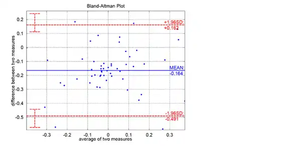
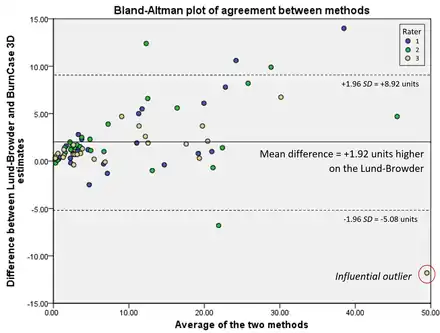
Bland–Altman plot
A Bland–Altman plot (difference plot) in analytical chemistry or biomedicine is a method of data plotting used in analyzing the agreement between two different assays. It is identical to a Tukey mean-difference plot,[1] the name by which it is known in other fields, but was popularised in medical statistics by J. Martin Bland and Douglas G. Altman.[2][3]

Agreement versus correlation
Bland and Altman make the point that any two methods that are designed to measure the same parameter (or property) should have good correlation when a set of samples are chosen such that the property to be determined varies considerably. A high correlation for any two methods designed to measure the same property could thus in itself just be a sign that one has chosen a widespread sample. A high correlation does not necessarily imply that there is good agreement between the two methods.
Construction
Consider a sample consisting of observations (for example, objects of unknown volume). Both assays (for example, different methods of volume measurement) are performed on each sample, resulting in data points. Each of the samples is then represented on the graph by assigning the mean of the two measurements as the -value, and the difference between the two values as the -value.
The Cartesian coordinates of a given sample with values of and determined by the two assays is
For comparing the dissimilarities between the two sets of samples independently from their mean values, it is more appropriate to look at the ratio of the pairs of measurements.[4] Log transformation (base 2) of the measurements before the analysis will enable the standard approach to be used; so the plot will be given by the following equation:
This version of the plot is used in MA plot.
Application
One primary application of the Bland–Altman plot is to compare two clinical measurements each of which produced some error in their measures.[5] It can also be used to compare a new measurement technique or method with a gold standard, as even a gold standard does not—and should not—imply it to be without error.[4] See Analyse-it, MedCalc, NCSS, GraphPad Prism, R, or StatsDirect for software providing Bland–Altman plots.
Bland–Altman plots are extensively used to evaluate the agreement among two different instruments or two measurements techniques. Bland–Altman plots allow identification of any systematic difference between the measurements (i.e., fixed bias) or possible outliers. The mean difference is the estimated bias, and the SD of the differences measures the random fluctuations around this mean. If the mean value of the difference differs significantly from 0 on the basis of a 1-sample t-test, this indicates the presence of fixed bias. If there is a consistent bias, it can be adjusted for by subtracting the mean difference from the new method. It is common to compute 95% limits of agreement for each comparison (average difference ± 1.96 standard deviation of the difference), which tells us how far apart measurements by two methods were more likely to be for most individuals. If the differences within mean ± 1.96 SD are not clinically important, the two methods may be used interchangeably. The 95% limits of agreement can be unreliable estimates of the population parameters especially for small sample sizes so, when comparing methods or assessing repeatability, it is important to calculate confidence intervals for 95% limits of agreement. This can be done by Bland and Altman's approximate method [3] or by more precise methods.[6]

Bland–Altman plots were also used to investigate any possible relationship of the discrepancies between the measurements and the true value (i.e., proportional bias). The existence of proportional bias indicates that the methods do not agree equally through the range of measurements (i.e., the limits of agreement will depend on the actual measurement). To evaluate this relationship formally, the difference between the methods should be regressed on the average of the 2 methods. When a relationship between the differences and the true value was identified (i.e., a significant slope of the regression line), regression-based 95% limits of agreement should be provided. [4]
Notes
A similar method was proposed in 1981 by Eksborg.[7] This method was based on Deming regression—a method introduced by Adcock in 1878.
Bland and Altman's Lancet paper [3] was number 29 in a list of the top 100 most-cited papers of all time with over 23,000 citations.[8]
See also
References
- Cleveland, William S. (1993). Visualizing data. Murray Hill, N.J.: At & T Bell Laboratories. pp. 22–23. ISBN 978-0963488404. OCLC 29456028.
- Altman DG, Bland JM (1983). "Measurement in medicine: the analysis of method comparison studies". The Statistician. 32 (3): 307–317. doi:10.2307/2987937. JSTOR 2987937.
- Bland JM, Altman DG (1986). "Statistical methods for assessing agreement between two methods of clinical measurement" (PDF). Lancet. 327 (8476): 307–10. CiteSeerX 10.1.1.587.8931. doi:10.1016/S0140-6736(86)90837-8. PMID 2868172. S2CID 2844897.
- Bland JM, Altman DG (1999). "Measuring agreement in method comparison studies". Statistical Methods in Medical Research. 8 (2): 135–60. doi:10.1177/096228029900800204. PMID 10501650. S2CID 9851097.
- Hanneman SK (2008). "Design, analysis, and interpretation of method-comparison studies". AACN Advanced Critical Care. 19 (2): 223–234. doi:10.1097/01.AACN.0000318125.41512.a3. PMC 2944826. PMID 18560291.
- Carkeet A (2015). "Exact parametric confidence intervals for Bland–Altman Limits of Agreement" (PDF). Optometry and Vision Science. 92 (3): e71–e80. doi:10.1097/OPX.0000000000000513. PMID 25650900. S2CID 11643889.
- Eksborg S (1981) Evaluation of method-comparison data. Clin Chem 27:1311–1312
- Van Noorden, Richard; Maher, Brendan; Nuzzo, Regina (2014). "The top 100 papers". Nature. 514 (7524): 550–553. doi:10.1038/514550a. ISSN 0028-0836. PMID 25355343.