Compositional data

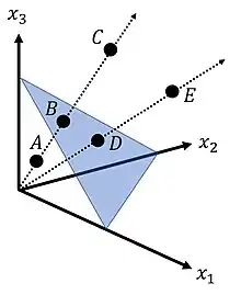
In statistics, compositional data are quantitative descriptions of the parts of some whole, conveying relative information. Mathematically, compositional data is represented by points on a simplex. Measurements involving probabilities, proportions, percentages, and ppm can all be thought of as compositional data.

Ternary plot

Compositional data in three variables can be plotted via ternary plots. The use of a barycentric plot on three variables graphically depicts the ratios of the three variables as positions in an equilateral triangle.

Simplicial sample space

In general, John Aitchison defined compositional data to be proportions of some whole in 1982.[1] In particular, a compositional data point (or composition for short) can be represented by a real vector with positive components. The sample space of compositional data is a simplex:

${\displaystyle {\mathcal {S}}^{D}=\left\{\mathbf {x} =[x_{1},x_{2},\dots ,x_{D}]\in \mathbb {R} ^{D}\,\left|\,x_{i}>0,i=1,2,\dots ,D;\sum _{i=1}^{D}x_{i}=\kappa \right.\right\}.\ }$

An illustration of the Aitchison simplex. Here, there are 3 parts, ${\displaystyle x_{1},x_{2},x_{3}}$ represent values of different proportions. A, B, C, D and E are 5 different compositions within the simplex. A, B and C are all equivalent and D and E are equivalent.

The only information is given by the ratios between components, so the information of a composition is preserved under multiplication by any positive constant. Therefore, the sample space of compositional data can always be assumed to be a standard simplex, i.e. ${\displaystyle \kappa =1}$. In this context, normalization to the standard simplex is called closure and is denoted by ${\displaystyle \scriptstyle {\mathcal {C}}[\,\cdot \,]}$:

${\displaystyle {\mathcal {C}}[x_{1},x_{2},\dots ,x_{D}]=\left[{\frac {x_{1}}{\sum _{i=1}^{D}x_{i}}},{\frac {x_{2}}{\sum _{i=1}^{D}x_{i}}},\dots ,{\frac {x_{D}}{\sum _{i=1}^{D}x_{i}}}\right],\ }$

where D is the number of parts (components) and ${\displaystyle [\cdot ]}$ denotes a row vector.

Aitchison geometry

The simplex can be given the structure of a real vector space in several different ways. The following vector space structure is called Aitchison geometry or the Aitchison simplex and has the following operations:

Perturbation

${\displaystyle x\oplus y=\left[{\frac {x_{1}y_{1}}{\sum _{i=1}^{D}x_{i}y_{i}}},{\frac {x_{2}y_{2}}{\sum _{i=1}^{D}x_{i}y_{i}}},\dots ,{\frac {x_{D}y_{D}}{\sum _{i=1}^{D}x_{i}y_{i}}}\right]=C[x_{1}y_{1},\ldots ,x_{D}y_{D}]\qquad \forall x,y\in S^{D}}$

Powering

${\displaystyle \alpha \odot x=\left[{\frac {x_{1}^{\alpha }}{\sum _{i=1}^{D}x_{i}^{\alpha }}},{\frac {x_{2}^{\alpha }}{\sum _{i=1}^{D}x_{i}^{\alpha }}},\ldots ,{\frac {x_{D}^{\alpha }}{\sum _{i=1}^{D}x_{i}^{\alpha }}}\right]=C[x_{1}^{\alpha },\ldots ,x_{D}^{\alpha }]\qquad \forall x\in S^{D},\;\alpha \in \mathbb {R} }$

Inner product

${\displaystyle \langle x,y\rangle ={\frac {1}{2D}}\sum _{i=1}^{D}\sum _{j=1}^{D}\log {\frac {x_{i}}{x_{j}}}\log {\frac {y_{i}}{y_{j}}}\qquad \forall x,y\in S^{D}}$

Under these operations alone, it is sufficient to show that the Aitchison simplex forms a ${\displaystyle (D-1)}$-dimensional Euclidean vector space.

Orthonormal bases

Since the Aitchison simplex forms a finite dimensional Hilbert space, it is possible to construct orthonormal bases in the simplex. Every composition ${\displaystyle x}$ can be decomposed as follows

${\displaystyle x=\bigoplus _{i=1}^{D}x_{i}^{*}\odot e_{i}}$

where ${\displaystyle e_{1},\ldots ,e_{D-1}}$ forms an orthonormal basis in the simplex.[2] The values ${\displaystyle x_{i}^{*},i=1,2,\ldots ,D-1}$ are the (orthonormal and Cartesian) coordinates of ${\displaystyle x}$ with respect to the given basis. They are called isometric log-ratio coordinates ${\displaystyle (\operatorname {ilr} )}$.

Linear transformations

There are three well-characterized isomorphisms that transform from the Aitchison simplex to real space. All of these transforms satisfy linearity and as given below

Additive logratio transform

The additive log ratio (alr) transform is an isomorphism where ${\displaystyle \operatorname {alr} :S^{D}\rightarrow \mathbb {R} ^{D-1}}$. This is given by

${\displaystyle \operatorname {alr} (x)=\left[\log {\frac {x_{1}}{x_{D}}}\cdots \log {\frac {x_{D-1}}{x_{D}}}\right]}$

The choice of denominator component is arbitrary, and could be any specified component. This transform is commonly used in chemistry with measurements such as pH. In addition, this is the transform most commonly used for multinomial logistic regression. The alr transform is not an isometry, meaning that distances on transformed values will not be equivalent to distances on the original compositions in the simplex.

Center logratio transform

The center log ratio (clr) transform is both an isomorphism and an isometry where ${\displaystyle \operatorname {clr} :S^{D}\rightarrow U,\quad U\subset \mathbb {R} ^{D}}$

${\displaystyle \operatorname {clr} (x)=\left[\log {\frac {x_{1}}{g(x)}}\cdots \log {\frac {x_{D}}{g(x)}}\right]}$

Where ${\displaystyle g(x)}$ is the geometric mean of ${\displaystyle x}$. The inverse of this function is also known as the softmax function commonly used in neural networks.

Isometric logratio transform

The isometric log ratio (ilr) transform is both an isomorphism and an isometry where ${\displaystyle \operatorname {ilr} :S^{D}\rightarrow \mathbb {R} ^{D-1}}$

${\displaystyle \operatorname {ilr} (x)={\big [}\langle x,e_{1}\rangle ,\ldots ,\langle x,e_{D-1}\rangle {\big ]}}$

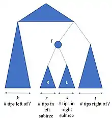
There are multiple ways to construct orthonormal bases, including using the Gram–Schmidt orthogonalization or singular-value decomposition of clr transformed data. Another alternative is to construct log contrasts from a bifurcating tree. If we are given a bifurcating tree, we can construct a basis from the internal nodes in the tree.

A representation of a tree in terms of its orthogonal components. l represents an internal node, an element of the orthonormal basis. This is a precursor to using the tree as a scaffold for the ilr transform

Each vector in the basis would be determined as follows

${\displaystyle e_{\ell }=C[\exp(\,\underbrace {0,\ldots ,0} _{k},\underbrace {a,\ldots ,a} _{r},\underbrace {b,\ldots ,b} _{s},\underbrace {0,\ldots ,0} _{t}\,)]}$

The elements within each vector are given as follows

${\displaystyle a={\frac {\sqrt {s}}{\sqrt {r(r+s)}}}\quad {\text{and}}\quad b={\frac {-{\sqrt {r}}}{\sqrt {s(r+s)}}}}$

where ${\displaystyle k,r,s,t}$ are the respective number of tips in the corresponding subtrees shown in the figure. It can be shown that the resulting basis is orthonormal[3]

Once the basis ${\displaystyle \Psi }$ is built, the ilr transform can be calculated as follows

${\displaystyle \operatorname {ilr} (x)=\operatorname {clr} (x)\Psi ^{T}}$

where each element in the ilr transformed data is of the following form

${\displaystyle b_{i}={\sqrt {\frac {rs}{r+s}}}\log {\frac {g(x_{R})}{g(x_{S})}}}$

where ${\displaystyle x_{R}}$ and ${\displaystyle x_{S}}$ are the set of values corresponding to the tips in the subtrees ${\displaystyle R}$ and ${\displaystyle S}$

Examples

• In chemistry, compositions can be expressed as molar concentrations of each component. As the sum of all concentrations is not determined, the whole composition of D parts is needed and thus expressed as a vector of D molar concentrations. These compositions can be translated into weight per cent multiplying each component by the appropriated constant.
• In demography, a town may be a compositional data point in a sample of towns; a town in which 35% of the people are Christians, 55% are Muslims, 6% are Jews, and the remaining 4% are others would correspond to the quadruple [0.35, 0.55, 0.06, 0.04]. A data set would correspond to a list of towns.
• In geology, a rock composed of different minerals may be a compositional data point in a sample of rocks; a rock of which 10% is the first mineral, 30% is the second, and the remaining 60% is the third would correspond to the triple [0.1, 0.3, 0.6]. A data set would contain one such triple for each rock in a sample of rocks.
• In high throughput sequencing, data obtained are typically transformed to relative abundances, rendering them compositional.
• In probability and statistics, a partition of the sampling space into disjoint events is described by the probabilities assigned to such events. The vector of D probabilities can be considered as a composition of D parts. As they add to one, one probability can be suppressed and the composition is completely determined.
• In a survey, the proportions of people positively answering some different items can be expressed as percentages. As the total amount is identified as 100, the compositional vector of D components can be defined using only D − 1 components, assuming that the remaining component is the percentage needed for the whole vector to add to 100.

See also

• Mixture model
• Response surface methodology
• Applications of simplices
• Ternary plot

Notes

1. Aitchison, John (1982). "The Statistical Analysis of Compositional Data". Journal of the Royal Statistical Society. Series B (Methodological). 44 (2): 139–177. doi:10.1111/j.2517-6161.1982.tb01195.x.
2. Egozcue et al.
3. Egozcue & Pawlowsky-Glahn 2005

References

• Aitchison, J. (2011) [1986], The Statistical Analysis of Compositional Data, Monographs on statistics and applied probability, Springer, ISBN 978-94-010-8324-9
• van den Boogaart, K. Gerald; Tolosana-Delgado, Raimon (2013), Analyzing Compositional Data with R, Springer, ISBN 978-3-642-36809-7
• Egozcue, Juan Jose; Pawlowsky-Glahn, Vera; Mateu-Figueras, Gloria; Barcelo-Vidal, Carles (2003), "Isometric logratio transformations for compositional data analysis", Mathematical Geology, 35 (3): 279–300, doi:10.1023/A:1023818214614, S2CID 122844634
• Egozcue, Juan Jose; Pawlowsky-Glahn, Vera (2005), "Groups of parts and their balances in compositional data analysis", Mathematical Geology, 37 (7): 795–828, doi:10.1007/s11004-005-7381-9, S2CID 53061345
• Pawlowsky-Glahn, Vera; Egozcue, Juan Jose; Tolosana-Delgado, Raimon (2015), Modeling and Analysis of Compositional Data, Wiley, doi:10.1002/9781119003144, ISBN 9781119003144

External links

• CoDaWeb – Compositional Data Website
• Pawlowsky-Glahn, V.; Egozcue, J.J.; Tolosana-Delgado, R. (2007). "Lecture Notes on Compositional Data Analysis". hdl:10256/297. Cite journal requires |journal= (help)
• Why, and How, Should Geologists Use Compositional Data Analysis (wikibook)