Large eddy simulation

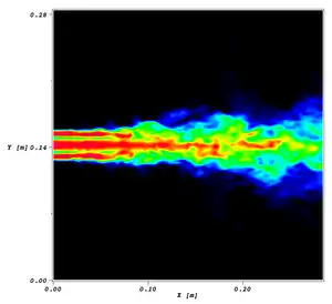
Large eddy simulation (LES) is a mathematical model for turbulence used in computational fluid dynamics. It was initially proposed in 1963 by Joseph Smagorinsky to simulate atmospheric air currents,[1] and first explored by Deardorff (1970).[2] LES is currently applied in a wide variety of engineering applications, including combustion,[3] acoustics,[4] and simulations of the atmospheric boundary layer.[5]

Large eddy simulation of a turbulent gas velocity field.

The simulation of turbulent flows by numerically solving the Navier–Stokes equations requires resolving a very wide range of time and length scales, all of which affect the flow field. Such a resolution can be achieved with direct numerical simulation (DNS), but DNS is computationally expensive, and its cost prohibits simulation of practical engineering systems with complex geometry or flow configurations, such as turbulent jets, pumps, vehicles, and landing gear.

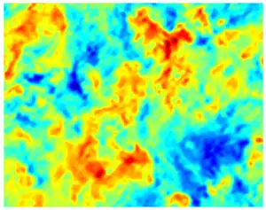
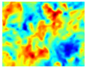
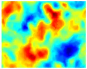
The principal idea behind LES is to reduce the computational cost by ignoring the smallest length scales, which are the most computationally expensive to resolve, via low-pass filtering of the Navier–Stokes equations. Such a low-pass filtering, which can be viewed as a time- and spatial-averaging, effectively removes small-scale information from the numerical solution. This information is not irrelevant, however, and its effect on the flow field must be modeled, a task which is an active area of research for problems in which small-scales can play an important role, such as near-wall flows [6][7] , reacting flows,[3] and multiphase flows.[8]

Filter definition and properties

A velocity field produced by a direct numerical simulation (DNS) of homogeneous decaying turbulence. The domain size is ${\displaystyle L^{3}}$.

The same DNS velocity field filtered using a box filter and ${\displaystyle \Delta =L/32}$.

The same DNS velocity field filtered using a box filter and ${\displaystyle \Delta =L/16}$.

An LES filter can be applied to a spatial and temporal field ${\displaystyle \phi ({\boldsymbol {x}},t)}$ and perform a spatial filtering operation, a temporal filtering operation, or both. The filtered field, denoted with a bar, is defined as:[9][10]

${\displaystyle {\overline {\phi ({\boldsymbol {x}},t)}}=\displaystyle {\int _{-\infty }^{\infty }}\int _{-\infty }^{\infty }\phi ({\boldsymbol {r}},\tau )G({\boldsymbol {x}}-{\boldsymbol {r}},t-\tau )d\tau d{\boldsymbol {r}}}$

where ${\displaystyle G}$ is the filter convolution kernel. This can also be written as:

${\displaystyle {\overline {\phi }}=G\star \phi .}$

The filter kernel ${\displaystyle G}$ has an associated cutoff length scale ${\displaystyle \Delta }$ and cutoff time scale ${\displaystyle \tau _{c}}$. Scales smaller than these are eliminated from ${\displaystyle {\overline {\phi }}}$. Using the above filter definition, any field ${\displaystyle \phi }$ may be split up into a filtered and sub-filtered (denoted with a prime) portion, as

${\displaystyle \phi ={\bar {\phi }}+\phi ^{\prime }.}$

It is important to note that the large eddy simulation filtering operation does not satisfy the properties of a Reynolds operator.

Filtered governing equations

The governing equations of LES are obtained by filtering the partial differential equations governing the flow field ${\displaystyle \rho {\boldsymbol {u}}({\boldsymbol {x}},t)}$. There are differences between the incompressible and compressible LES governing equations, which lead to the definition of a new filtering operation.

Incompressible flow

For incompressible flow, the continuity equation and Navier–Stokes equations are filtered, yielding the filtered incompressible continuity equation,

${\displaystyle {\frac {\partial {\bar {u_{i}}}}{\partial x_{i}}}=0}$

and the filtered Navier–Stokes equations,

${\displaystyle {\frac {\partial {\bar {u_{i}}}}{\partial t}}+{\frac {\partial }{\partial x_{j}}}\left({\overline {u_{i}u_{j}}}\right)=-{\frac {1}{\rho }}{\frac {\partial {\overline {p}}}{\partial x_{i}}}+\nu {\frac {\partial }{\partial x_{j}}}\left({\frac {\partial {\bar {u_{i}}}}{\partial x_{j}}}+{\frac {\partial {\bar {u_{j}}}}{\partial x_{i}}}\right)=-{\frac {1}{\rho }}{\frac {\partial {\overline {p}}}{\partial x_{i}}}+2\nu {\frac {\partial }{\partial x_{j}}}S_{ij},}$

where ${\displaystyle {\bar {p}}}$ is the filtered pressure field and ${\displaystyle S_{ij}}$ is the rate-of-strain tensor. The nonlinear filtered advection term ${\displaystyle {\overline {u_{i}u_{j}}}}$ is the chief cause of difficulty in LES modeling. It requires knowledge of the unfiltered velocity field, which is unknown, so it must be modeled. The analysis that follows illustrates the difficulty caused by the nonlinearity, namely, that it causes interaction between large and small scales, preventing separation of scales.

The filtered advection term can be split up, following Leonard (1974),[11] as:

${\displaystyle {\overline {u_{i}u_{j}}}=\tau _{ij}^{r}+{\overline {u}}_{i}{\overline {u}}_{j}}$

where ${\displaystyle \tau _{ij}^{r}}$ is the residual stress tensor, so that the filtered Navier Stokes equations become

${\displaystyle {\frac {\partial {\bar {u_{i}}}}{\partial t}}+{\frac {\partial }{\partial x_{j}}}\left({\overline {u}}_{i}{\overline {u}}_{j}\right)=-{\frac {1}{\rho }}{\frac {\partial {\overline {p}}}{\partial x_{i}}}+2\nu {\frac {\partial }{\partial x_{j}}}{\bar {S}}_{ij}-{\frac {\partial \tau _{ij}^{r}}{\partial x_{j}}}}$

with the residual stress tensor ${\displaystyle \tau _{ij}^{r}}$ grouping all unclosed terms. Leonard decomposed this stress tensor as ${\displaystyle \tau _{ij}^{r}=L_{ij}+C_{ij}+R_{ij}}$ and provided physical interpretations for each term. ${\displaystyle L_{ij}}$, the Leonard tensor, represents interactions among large scales, ${\displaystyle R_{ij}}$, the Reynolds stress-like term, represents interactions among the sub-filter scales (SFS), and ${\displaystyle C_{ij}}$, the Clark tensor,[12] represents cross-scale interactions between large and small scales.[11] Modeling the unclosed term ${\displaystyle \tau _{ij}^{r}}$ is the task of SFS models (also referred to as sub-grid scale, or SGS, models). This is made challenging by the fact that the sub-filter scale stress tensor ${\displaystyle \tau _{ij}^{r}}$ must account for interactions among all scales, including filtered scales with unfiltered scales.

The filtered governing equation for a passive scalar ${\displaystyle \phi }$, such as mixture fraction or temperature, can be written as

${\displaystyle {\frac {\partial {\overline {\phi }}}{\partial t}}+{\frac {\partial }{\partial x_{j}}}\left({\overline {u}}_{j}{\overline {\phi }}\right)={\frac {\partial {\overline {J_{\phi }}}}{\partial x_{j}}}+{\frac {\partial q_{j}}{\partial x_{j}}}}$

where ${\displaystyle J_{\phi }}$ is the diffusive flux of ${\displaystyle \phi }$, and ${\displaystyle q_{j}}$ is the sub-filter flux for the scalar ${\displaystyle \phi }$. The filtered diffusive flux ${\displaystyle {\overline {J_{\phi }}}}$ is unclosed, unless a particular form is assumed for it (e.g. a gradient diffusion model ${\displaystyle J_{\phi }=D_{\phi }{\frac {\partial \phi }{\partial x_{i}}}}$). ${\displaystyle q_{j}}$ is defined analogously to ${\displaystyle \tau _{ij}^{r}}$,

${\displaystyle q_{j}={\bar {\phi }}{\overline {u}}_{j}-{\overline {\phi u_{j}}}}$

and can similarly be split up into contributions from interactions between various scales. This sub-filter flux also requires a sub-filter model.

Derivation

Using Einstein notation, the Navier–Stokes equations for an incompressible fluid in Cartesian coordinates are

${\displaystyle {\frac {\partial u_{i}}{\partial x_{i}}}=0}$

${\displaystyle {\frac {\partial u_{i}}{\partial t}}+{\frac {\partial u_{i}u_{j}}{\partial x_{j}}}=-{\frac {1}{\rho }}{\frac {\partial p}{\partial x_{i}}}+\nu {\frac {\partial ^{2}u_{i}}{\partial x_{j}\partial x_{j}}}.}$

Filtering the momentum equation results in

${\displaystyle {\overline {\frac {\partial u_{i}}{\partial t}}}+{\overline {\frac {\partial u_{i}u_{j}}{\partial x_{j}}}}=-{\overline {{\frac {1}{\rho }}{\frac {\partial p}{\partial x_{i}}}}}+{\overline {\nu {\frac {\partial ^{2}u_{i}}{\partial x_{j}\partial x_{j}}}}}.}$

If we assume that filtering and differentiation commute, then

${\displaystyle {\frac {\partial {\bar {u_{i}}}}{\partial t}}+{\overline {\frac {\partial u_{i}u_{j}}{\partial x_{j}}}}=-{\frac {1}{\rho }}{\frac {\partial {\bar {p}}}{\partial x_{i}}}+\nu {\frac {\partial ^{2}{\bar {u_{i}}}}{\partial x_{j}\partial x_{j}}}.}$

This equation models the changes in time of the filtered variables ${\displaystyle {\bar {u_{i}}}}$. Since the unfiltered variables ${\displaystyle u_{i}}$ are not known, it is impossible to directly calculate ${\displaystyle {\overline {\frac {\partial u_{i}u_{j}}{\partial x_{j}}}}}$. However, the quantity ${\displaystyle {\frac {\partial {\bar {u_{i}}}{\bar {u_{j}}}}{\partial x_{j}}}}$ is known. A substitution is made:

${\displaystyle {\frac {\partial {\bar {u_{i}}}}{\partial t}}+{\frac {\partial {\bar {u_{i}}}{\bar {u_{j}}}}{\partial x_{j}}}=-{\frac {1}{\rho }}{\frac {\partial {\bar {p}}}{\partial x_{i}}}+\nu {\frac {\partial ^{2}{\bar {u_{i}}}}{\partial x_{j}\partial x_{j}}}-\left({\overline {\frac {\partial u_{i}u_{j}}{\partial x_{j}}}}-{\frac {\partial {\bar {u_{i}}}{\bar {u_{j}}}}{\partial x_{j}}}\right).}$

Let ${\displaystyle \tau _{ij}={\overline {u_{i}u_{j}}}-{\bar {u_{i}}}{\bar {u_{j}}}}$. The resulting set of equations are the LES equations:

${\displaystyle {\frac {\partial {\bar {u_{i}}}}{\partial t}}+{\bar {u_{j}}}{\frac {\partial {\bar {u_{i}}}}{\partial x_{j}}}=-{\frac {1}{\rho }}{\frac {\partial {\bar {p}}}{\partial x_{i}}}+\nu {\frac {\partial ^{2}{\bar {u_{i}}}}{\partial x_{j}\partial x_{j}}}-{\frac {\partial \tau _{ij}}{\partial x_{j}}}.}$

Compressible governing equations

For the governing equations of compressible flow, each equation, starting with the conservation of mass, is filtered. This gives:

${\displaystyle {\frac {\partial {\overline {\rho }}}{\partial t}}+{\frac {\partial {\overline {u_{i}\rho }}}{\partial x_{i}}}=0}$

which results in an additional sub-filter term. However, it is desirable to avoid having to model the sub-filter scales of the mass conservation equation. For this reason, Favre[13] proposed a density-weighted filtering operation, called Favre filtering, defined for an arbitrary quantity ${\displaystyle \phi }$ as:

${\displaystyle {\tilde {\phi }}={\frac {\overline {\rho \phi }}{\overline {\rho }}}}$

which, in the limit of incompressibility, becomes the normal filtering operation. This makes the conservation of mass equation:

${\displaystyle {\frac {\partial {\overline {\rho }}}{\partial t}}+{\frac {\partial {\overline {\rho }}{\tilde {u_{i}}}}{\partial x_{i}}}=0.}$

This concept can then be extended to write the Favre-filtered momentum equation for compressible flow. Following Vreman:[14]

${\displaystyle {\frac {\partial {\overline {\rho }}{\tilde {u_{i}}}}{\partial t}}+{\frac {\partial {\overline {\rho }}{\tilde {u_{i}}}{\tilde {u_{j}}}}{\partial x_{j}}}+{\frac {\partial {\overline {p}}}{\partial x_{i}}}-{\frac {\partial {\tilde {\sigma }}_{ij}}{\partial x_{j}}}=-{\frac {\partial {\overline {\rho }}\tau _{ij}^{r}}{\partial x_{j}}}+{\frac {\partial }{\partial x_{j}}}\left({\overline {\sigma }}_{ij}-{\tilde {\sigma }}_{ij}\right)}$

where ${\displaystyle \sigma _{ij}}$ is the shear stress tensor, given for a Newtonian fluid by:

${\displaystyle \sigma _{ij}=2\mu (T)S_{ij}-{\frac {2}{3}}\mu (T)\delta _{ij}S_{kk}}$

and the term ${\displaystyle {\frac {\partial }{\partial x_{j}}}\left({\overline {\sigma }}_{ij}-{\tilde {\sigma }}_{ij}\right)}$ represents a sub-filter viscous contribution from evaluating the viscosity ${\displaystyle \mu (T)}$ using the Favre-filtered temperature ${\displaystyle {\tilde {T}}}$. The subgrid stress tensor for the Favre-filtered momentum field is given by

${\displaystyle \tau _{ij}^{r}={\widetilde {u_{i}\cdot u_{j}}}-{\tilde {u_{i}}}{\tilde {u_{j}}}}$

By analogy, the Leonard decomposition may also be written for the residual stress tensor for a filtered triple product ${\displaystyle {\overline {\rho \phi \psi }}}$. The triple product can be rewritten using the Favre filtering operator as ${\displaystyle {\overline {\rho }}{\widetilde {\phi \psi }}}$, which is an unclosed term (it requires knowledge of the fields ${\displaystyle \phi }$ and ${\displaystyle \psi }$, when only the fields ${\displaystyle {\tilde {\phi }}}$ and ${\displaystyle {\tilde {\psi }}}$ are known). It can be broken up in a manner analogous to ${\displaystyle {\overline {u_{i}u_{j}}}}$ above, which results in a sub-filter stress tensor ${\displaystyle {\overline {\rho }}\left({\widetilde {\phi \psi }}-{\tilde {\phi }}{\tilde {\psi }}\right)}$. This sub-filter term can be split up into contributions from three types of interactions: the Leondard tensor ${\displaystyle L_{ij}}$, representing interactions among resolved scales; the Clark tensor ${\displaystyle C_{ij}}$, representing interactions between resolved and unresolved scales; and the Reynolds tensor ${\displaystyle R_{ij}}$, which represents interactions among unresolved scales.[15]

Filtered kinetic energy equation

In addition to the filtered mass and momentum equations, filtering the kinetic energy equation can provide additional insight. The kinetic energy field can be filtered to yield the total filtered kinetic energy:

${\displaystyle {\overline {E}}={\frac {1}{2}}{\overline {u_{i}u_{i}}}}$

and the total filtered kinetic energy can be decomposed into two terms: the kinetic energy of the filtered velocity field ${\displaystyle E_{f}}$,

${\displaystyle E_{f}={\frac {1}{2}}{\overline {u_{i}}}\,{\overline {u_{i}}}}$

and the residual kinetic energy ${\displaystyle k_{r}}$,

${\displaystyle k_{r}={\frac {1}{2}}{\overline {u_{i}u_{i}}}-{\frac {1}{2}}{\overline {u_{i}}}\,{\overline {u_{i}}}={\frac {1}{2}}\tau _{ii}^{r}}$

such that ${\displaystyle {\overline {E}}=E_{f}+k_{r}}$.

The conservation equation for ${\displaystyle E_{f}}$ can be obtained by multiplying the filtered momentum transport equation by ${\displaystyle {\overline {u_{i}}}}$ to yield:

${\displaystyle {\frac {\partial E_{f}}{\partial t}}+{\overline {u_{j}}}{\frac {\partial E_{f}}{\partial x_{j}}}+{\frac {1}{\rho }}{\frac {\partial {\overline {u_{i}}}{\bar {p}}}{\partial x_{i}}}+{\frac {\partial {\overline {u_{i}}}\tau _{ij}^{r}}{\partial x_{j}}}-2\nu {\frac {\partial {\overline {u_{i}}}{\bar {S_{ij}}}}{\partial x_{j}}}=-\epsilon _{f}-\Pi }$

where ${\displaystyle \epsilon _{f}=2\nu {\bar {S_{ij}}}{\bar {S_{ij}}}}$ is the dissipation of kinetic energy of the filtered velocity field by viscous stress, and ${\displaystyle \Pi =-\tau _{ij}^{r}{\bar {S_{ij}}}}$ represents the sub-filter scale (SFS) dissipation of kinetic energy.

The terms on the left-hand side represent transport, and the terms on the right-hand side are sink terms that dissipate kinetic energy.[9]

The ${\displaystyle \Pi }$ SFS dissipation term is of particular interest, since it represents the transfer of energy from large resolved scales to small unresolved scales. On average, ${\displaystyle \Pi }$ transfers energy from large to small scales. However, instantaneously ${\displaystyle \Pi }$ can be positive or negative, meaning it can also act as a source term for ${\displaystyle E_{f}}$, the kinetic energy of the filtered velocity field. The transfer of energy from unresolved to resolved scales is called backscatter (and likewise the transfer of energy from resolved to unresolved scales is called forward-scatter).[16]

Numerical methods for LES

Large eddy simulation involves the solution to the discrete filtered governing equations using computational fluid dynamics. LES resolves scales from the domain size ${\displaystyle L}$ down to the filter size ${\displaystyle \Delta }$, and as such a substantial portion of high wave number turbulent fluctuations must be resolved. This requires either high-order numerical schemes, or fine grid resolution if low-order numerical schemes are used. Chapter 13 of Pope[9] addresses the question of how fine a grid resolution ${\displaystyle \Delta x}$ is needed to resolve a filtered velocity field ${\displaystyle {\overline {u}}({\boldsymbol {x}})}$. Ghosal[17] found that for low-order discretization schemes, such as those used in finite volume methods, the truncation error can be the same order as the subfilter scale contributions, unless the filter width ${\displaystyle \Delta }$ is considerably larger than the grid spacing ${\displaystyle \Delta x}$. While even-order schemes have truncation error, they are non-dissipative,[18] and because subfilter scale models are dissipative, even-order schemes will not affect the subfilter scale model contributions as strongly as dissipative schemes.

Filter implementation

The filtering operation in large eddy simulation can be implicit or explicit. Implicit filtering recognizes that the subfilter scale model will dissipate in the same manner as many numerical schemes. In this way, the grid, or the numerical discretization scheme, can be assumed to be the LES low-pass filter. While this takes full advantage of the grid resolution, and eliminates the computational cost of calculating a subfilter scale model term, it is difficult to determine the shape of the LES filter that is associated with some numerical issues. Additionally, truncation error can also become an issue.[19]

In explicit filtering, an LES filter is applied to the discretized Navier–Stokes equations, providing a well-defined filter shape and reducing the truncation error. However, explicit filtering requires a finer grid than implicit filtering, and the computational cost increases with ${\displaystyle (\Delta x)^{4}}$. Chapter 8 of Sagaut (2006) covers LES numerics in greater detail.[10]

Boundary conditions of large eddy simulations

Inlet boundary conditions affect the accuracy of LES significantly, and the treatment of inlet conditions for LES is a complicated problem. Theoretically, a good boundary condition for LES should contain the following features:[20]

(1) providing accurate information of flow characteristics, i.e. velocity and turbulence;

(2) satisfying the Navier-Stokes equations and other physics;

(3) being easy to implement and adjust to different cases.

Currently, methods of generating inlet conditions for LES are broadly divided into two categories classified by Tabor et al.:[21]

The first method for generating turbulent inlets is to synthesize them according to particular cases, such as Fourier techniques, principle orthogonal decomposition (POD) and vortex methods. The synthesis techniques attempt to construct turbulent field at inlets that have suitable turbulence-like properties and make it easy to specify parameters of the turbulence, such as turbulent kinetic energy and turbulent dissipation rate. In addition, inlet conditions generated by using random numbers are computationally inexpensive. However, one serious drawback exists in the method. The synthesized turbulence does not satisfy the physical structure of fluid flow governed by Navier-Stokes equations.[20]

The second method involves a separate and precursor calculation to generate a turbulent database which can be introduced into the main computation at the inlets. The database (sometimes named as ‘library’) can be generated in a number of ways, such as cyclic domains, pre-prepared library, and internal mapping. However, the method of generating turbulent inflow by precursor simulations requires large calculation capacity.

Researchers examining the application of various types of synthetic and precursor calculations have found that the more realistic the inlet turbulence, the more accurate LES predicts results.[20]

Modeling unresolved scales

To discuss the modeling of unresolved scales, first the unresolved scales must be classified. They fall into two groups: resolved sub-filter scales (SFS), and sub-grid scales(SGS).

The resolved sub-filter scales represent the scales with wave numbers larger than the cutoff wave number ${\displaystyle k_{c}}$, but whose effects are dampened by the filter. Resolved sub-filter scales only exist when filters non-local in wave-space are used (such as a box or Gaussian filter). These resolved sub-filter scales must be modeled using filter reconstruction.

Sub-grid scales are any scales that are smaller than the cutoff filter width ${\displaystyle \Delta }$. The form of the SGS model depends on the filter implementation. As mentioned in the Numerical methods for LES section, if implicit LES is considered, no SGS model is implemented and the numerical effects of the discretization are assumed to mimic the physics of the unresolved turbulent motions.

Sub-grid scale models

Without a universally valid description of turbulence, empirical information must be utilized when constructing and applying SGS models, supplemented with fundamental physical constraints such as Galilean invariance[9] .[22] Two classes of SGS models exist; the first class is functional models and the second class is structural models. Some models may be categorized as both.

Functional (eddy–viscosity) models

Functional models are simpler than structural models, focusing only on dissipating energy at a rate that is physically correct. These are based on an artificial eddy viscosity approach, where the effects of turbulence are lumped into a turbulent viscosity. The approach treats dissipation of kinetic energy at sub-grid scales as analogous to molecular diffusion. In this case, the deviatoric part of ${\displaystyle \tau _{ij}}$ is modeled as:

${\displaystyle \tau _{ij}^{r}-{\frac {1}{3}}\tau _{kk}\delta _{ij}=-2\nu _{\mathrm {t} }{\bar {S}}_{ij}}$

where ${\displaystyle \nu _{\mathrm {t} }}$ is the turbulent eddy viscosity and ${\displaystyle {\bar {S}}_{ij}={\frac {1}{2}}\left({\frac {\partial {\bar {u}}_{i}}{\partial x_{j}}}+{\frac {\partial {\bar {u}}_{j}}{\partial x_{i}}}\right)}$ is the rate-of-strain tensor.

Based on dimensional analysis, the eddy viscosity must have units of ${\displaystyle \left[\nu _{\mathrm {t} }\right]={\frac {\mathrm {m^{2}} }{\mathrm {s} }}}$. Most eddy viscosity SGS models model the eddy viscosity as the product of a characteristic length scale and a characteristic velocity scale.

Smagorinsky–Lilly model

The first SGS model developed was the Smagorinsky–Lilly SGS model, which was developed by Smagorinsky[1] and used in the first LES simulation by Deardorff.[2] It models the eddy viscosity as:

${\displaystyle \nu _{\mathrm {t} }=(C_{s}\Delta _{g})^{2}{\sqrt {2{\bar {S}}_{ij}{\bar {S}}_{ij}}}=(C_{s}\Delta _{g})^{2}\left|S\right|}$

where ${\displaystyle \Delta _{g}}$ is the grid size and ${\displaystyle C_{s}}$ is a constant.

This method assumes that the energy production and dissipation of the small scales are in equilibrium - that is, ${\displaystyle \epsilon =\Pi }$.

Germano dynamic model

Germano et al.[23] identified a number of studies using the Smagorinsky model that each found different values for the Smagorinsky constant ${\displaystyle C_{s}}$ for different flow configurations. In an attempt to formulate a more universal approach to SGS models, Germano et al. proposed a dynamic Smagorinsky model, which utilized two filters: a grid LES filter, denoted ${\displaystyle {\overline {\cdot }}}$, and a test LES filter, denoted ${\displaystyle {\hat {\cdot }}}$. In this case, the resolved turbulent stress tensor ${\displaystyle {\mathcal {L}}_{ij}}$ is defined as

${\displaystyle {\mathcal {L}}_{ij}=T_{ij}^{r}-{\hat {\tau }}_{ij}^{r}}$

which is also called the Germano identity. The quantity ${\displaystyle T_{ij}^{r}={\widehat {\overline {u_{i}u_{j}}}}-{\hat {\bar {u}}}_{i}{\hat {\bar {u}}}_{j}}$ is the residual stress tensor for the test filter scale, and ${\displaystyle {\hat {\tau }}_{ij}^{r}={\widehat {\overline {u_{i}u_{j}}}}-{\widehat {{\overline {u}}_{i}{\overline {u}}_{j}}}}$ is the residual stress tensor for the grid filter, then test filtered.

${\displaystyle {\mathcal {L}}_{ij}}$ represents the contribution to the SGS stresses by length scales smaller than the test filter width ${\displaystyle {\hat {\Delta }}}$ but larger than the grid filter width ${\displaystyle {\overline {\Delta }}}$. The dynamic model then finds the coefficient that best complies with the Germano identity. However, since the identity is a tensorial equation, it is overdetermined (five equations for one unknown), prompting Lilly [24] to propose a minimum least-square error method that leads to an equation for ${\displaystyle C_{s}}$:

${\displaystyle C_{s}^{2}={\frac {{\mathcal {L}}_{ij}{\mathcal {M}}_{ij}}{{\mathcal {M}}_{ij}{\mathcal {M}}_{ij}}}}$

where

${\displaystyle {\mathcal {M}}_{ij}=2{\overline {\Delta }}^{2}\left({\overline {\left|{\hat {S}}\right|{\hat {S}}_{ij}}}-\alpha ^{2}\left|{\overline {\hat {S}}}\right|{\overline {\hat {S}}}_{ij}\right)}$ and ${\displaystyle \alpha ={\hat {\Delta }}/{\overline {\Delta }}.}$

However, this procedure was numerically unstable since the numerator could become negative and large fluctuations in ${\displaystyle C_{s}}$ were often observed. Hence, additional averaging of the error in the minimization is often employed, leading to:

${\displaystyle C_{s}^{2}={\frac {\left\langle {\mathcal {L}}_{ij}{\mathcal {M}}_{ij}\right\rangle }{\left\langle {\mathcal {M}}_{ij}{\mathcal {M}}_{ij}\right\rangle }}}$

This has made the dynamic model more stable and making the method more widely applicable. Inherent in the procedure is the assumption that the coefficient ${\displaystyle C_{s}}$ is invariant of scale (see review [25]). The averaging can be a spatial averaging over directions of statistical homogeneity (e.g. volume for homogeneous turbulence or wall-parallel planes for channel flow as originally used in Germano et al.[23]), or time following Lagrangian fluid trajectories .[26]

See also

• Direct numerical simulation
• Fluid mechanics
• Galilean invariance – an important property of certain types of filters
• Reynolds-averaged Navier–Stokes equations
• Turbulence

Further reading

• Heus, T.; van Heerwaarden, C. C.;Jonker, H. J. J.; Pier Siebesma, A.; Axelsen, S.«Formulation of the Dutch Atmospheric Large-Eddy Simulation (DALES) and overview of its applications» Geoscientific Model Development, 3, 2, 30-09-2010, pàg. 415–444. DOI: 10.5194/gmd-3-415-2010. ISSN: 1991-9603.

References

1. Smagorinsky, Joseph (March 1963). "General Circulation Experiments with the Primitive Equations". Monthly Weather Review. 91 (3): 99–164. Bibcode:1963MWRv...91...99S. doi:10.1175/1520-0493(1963)091<0099:GCEWTP>2.3.CO;2.
2. Deardorff, James (1970). "A numerical study of three-dimensional turbulent channel flow at large Reynolds numbers". Journal of Fluid Mechanics. 41 (2): 453–480. Bibcode:1970JFM....41..453D. doi:10.1017/S0022112070000691.
3. Pitsch, Heinz (2006). "Large-Eddy Simulation of Turbulent Combustion" (PDF). Annual Review of Fluid Mechanics. 38 (1): 453–482. Bibcode:2006AnRFM..38..453P. doi:10.1146/annurev.fluid.38.050304.092133.
4. Wagner, Claus; Hüttl, Thomas; Sagaut, Pierre (2007). Large-Eddy Simulation for Acoustics. Cambridge University Press. ISBN 978-0-521-87144-0.
5. Sullivan, Peter P.; McWilliams, James C.; Moeng, Chin-Hoh (1994). "A subgrid-scale model for large-eddy simulation of planetary boundary-layer flows". Boundary-Layer Meteorology. 71 (3): 247–276. Bibcode:1994BoLMe..71..247S. CiteSeerX 10.1.1.463.6006. doi:10.1007/BF00713741. ISSN 0006-8314.
6. Piomelli, Ugo; Elias Balaras (2002). "Wall-layer models for large-eddy simulations". Annual Review of Fluid Mechanics. 34 (34): 349–374. Bibcode:2002AnRFM..34..349P. doi:10.1146/annurev.fluid.34.082901.144919.
7. Spalart, P. R. (2009). "Detached-eddy simulation". Annual Review of Fluid Mechanics. 41 (1): 181–202. Bibcode:2009AnRFM..41..181S. doi:10.1146/annurev.fluid.010908.165130.
8. Fox, R. O. (2012). "Large-eddy-simulation tools for multiphase flows". Annual Review of Fluid Mechanics. 44 (1): 47–76. Bibcode:2012AnRFM..44...47F. doi:10.1146/annurev-fluid-120710-101118.
9. Pope, S. B. (2000). Turbulent Flows. Cambridge University Press.
10. Sagaut, Pierre (2006). Large Eddy Simulation for Incompressible Flows (Third ed.). Springer. ISBN 978-3-540-26344-9.
11. Leonard, A. (1974). Energy cascade in large-eddy simulations of turbulent fluid flows. Advances in Geophysics A. Advances in Geophysics. 18. pp. 237–248. Bibcode:1975AdGeo..18..237L. doi:10.1016/S0065-2687(08)60464-1. ISBN 9780120188185.
12. Clark, R.; Ferziger, J.; Reynolds, W. (1979). "Evaluation of subgrid-scale models using an accurately simulated turbulent flow". Journal of Fluid Mechanics. 91: 1–16. Bibcode:1979JFM....91....1C. doi:10.1017/S002211207900001X.
13. Favre, Alexandre (1983). "Turbulence: space-time statistical properties and behavior in supersonic flows". Physics of Fluids A. 23 (10): 2851–2863. Bibcode:1983PhFl...26.2851F. doi:10.1063/1.864049.
14. Vreman, Bert; Geurts, Bernard; Kuerten, Hans (1995). "Subgrid-modelling in LES of compressible flow". Applied Scientific Research. 45 (3): 191–203. doi:10.1007/BF00849116.
15. Garnier, E.; Adams, N.; Sagaut, P. (2009). Large eddy simulation for compressible flows. Springer. doi:10.1007/978-90-481-2819-8. ISBN 978-90-481-2818-1.
16. Piomelli, U.; Cabot, W.; Moin, P.; Lee, S. (1991). "Subgrid-scale backscatter in turbulent and transitional flows". Physics of Fluids A. 3 (7): 1766–1771. Bibcode:1991PhFl....3.1766P. doi:10.1063/1.857956.
17. Ghosal, S. (April 1996). "An analysis of numerical errors in large-eddy simulations of turbulence". Journal of Computational Physics. 125 (1): 187–206. Bibcode:1996JCoPh.125..187G. doi:10.1006/jcph.1996.0088.
18. Randall J. Leveque (1992). Numerical Methods for Conservation Laws (2nd ed.). Birkhäuser Basel. ISBN 978-3-7643-2723-1.
19. Grinstein, Fernando; Margolin, Len; Rider, William (2007). Implicit large eddy simulation. Cambridge University Press. ISBN 978-0-521-86982-9.
20. Li, P., Eckels, S., Mann, G., Zhang, N. A Method of Measuring Turbulent Flow Structures With Particle Image Velocimetry and Incorporating Into Boundary Conditions of Large Eddy Simulations. ASME. J. Fluids Eng. 2018;140(7):071401-071401-11. doi:10.1115/1.4039256.
21. Tabor, G. R., & Baba-Ahmadi, M. H. (2010). Inlet conditions for large eddy simulation: a review. Computers & Fluids, 39(4), 553-567.
22. Meneveau, C. (2010). "Turbulence: Subgrid-Scale Modeling". Scholarpedia. 5 (1): 9489. Bibcode:2010SchpJ...5.9489M. doi:10.4249/scholarpedia.9489.
23. Germano, M.; Piomelli, U.; Moin, P.; Cabot, W. (1991). "A dynamic subgrid‐scale eddy viscosity model". Physics of Fluids A. 3 (7): 1760–1765. Bibcode:1991PhFl....3.1760G. doi:10.1063/1.857955.
24. Lilly, D. K. (1992). "A proposed modification of the Germano subgrid-scale closure method". Physics of Fluids A. 4 (3): 633–636. Bibcode:1992PhFlA...4..633L. doi:10.1063/1.858280.
25. Meneveau, C.; Katz, J. (2000). "Scale-Invariance and Turbulence Models for Large-Eddy Simulation". Annu. Rev. Fluid Mech. 32 (1): 1–32. Bibcode:2000AnRFM..32....1M. doi:10.1146/annurev.fluid.32.1.1.
26. Meneveau, C.; Lund, T. S.; Cabot, W. H. (1996). "A Lagrangian dynamic subgrid-scale model of turbulence". J. Fluid Mech. 319 (1): 353–385. Bibcode:1996JFM...319..353M. doi:10.1017/S0022112096007379. hdl:2060/19950014634.