MLAB
MLAB (Modeling LABoratory) is a multi-paradigm numerical computing environment and fourth-generation programming language.
 | |
| Developer(s) | Civilized Software Inc. |
|---|---|
| Initial release | 1985 |
| Written in | C, Assembler, MLAB [1] |
| Operating system | Cross-platform: Microsoft Windows, Linux, and Mac OS X |
| Platform | IA-32, x86-64 |
| Type | Numerical computing |
| License | Proprietary commercial software |
| Website | www |
| Paradigm | multi-paradigm: functional, imperative, procedural, array |
|---|---|
| Designed by | Gary D. Knott, Daniel R. Kerner, and Barry Bunow |
| Developer | Civilized Software |
| First appeared | late 1970s |
| Typing discipline | dynamic, weak |
| OS | Cross-platform |
| Website | www |
| |
A proprietary programming language developed by Civilized Software, Inc., MLAB allows matrix manipulations, plotting of functions and data, and implementation of algorithms, and provides support for curve-fitting, differential equations, statistics and graphics.
MLAB is intended for numerical computing, with special facilities for ordinary differential equation-solving (ODE-solving) and curve-fitting (non-linear regression.) It provides more than thirty command types and more than 450 built-in functions from the areas of elementary mathematics, transcendental functions, probability and statistics, linear algebra, optimization, cluster analysis, combinatorics, numeric input/output, and graphics.
The usual low-level functions, e.g. sine, cosine, log, etc., are present, as well as functions performing more complex analyses, such as singular value decomposition, discrete Fourier transforms, solution of differential equation systems, non-parametric modeling and constrained non-linear optimization, among many others. A substantial collection of statistically-oriented functions, such as most common distribution functions and their inverses, are included, as well as robust graph creation features, supporting graphing of exceptionally complex functions.
Many software packages can integrate ordinary differential equations numerically, but MLAB is one of the very few that also can adjust parameters and initial conditions. MLAB is equally facile at handling curve fitting, where the adjustments are linear or, as is the case with most differential equation models, nonlinear.
MLAB is widely used in academic and research institutions as well as industrial enterprises.
History
MLAB was originally developed at the National Institute of Health in the late 1970s using Stanford's SAIL running on Digital Equipment Corporation (DEC) PDP-10 computers. The creators of MLAB founded Civilized Software, Inc. in 1985 and expanded MLAB in the late 1980s and early 1990s through the application of Small Business Innovation Research grants.
MLAB was first adopted by researchers and practitioners in biochemistry, but quickly spread to many other domains. It is now also used in education, in particular the teaching of linear algebra, numerical analysis, and is popular amongst scientists involved in chemical kinetics analysis and modeling[2] and compartmental modeling in pharmacological (including pharmacokinetics) and physiological research.
Syntax
The MLAB application is built around the MLAB scripting language. Common usage of the MLAB application involves using the Command Window as an interactive mathematical or executing text (script) files containing MLAB code.
There are dozens of MLAB commands and hundreds of MLAB functions. In essence, MLAB is an interpreter for a high-level mathematical language with the ability to process re-runnable script files called do-files.
Example
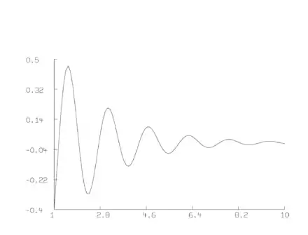
In MLAB one can define a function and graph it as follows.
 function f(x) = a*cos(b*x)*exp(-k*x)
 a = 1; b=4; k =.5
 v=1:10!100
 m= points(f,v)
 draw m
 view
The result is a simple plot:

Note that 1:10!100 = 1:10:0.0909090909, which means that we are dealing with a column vector of values from 1 to 10 in steps of size 0.0909090909
Also, note that points(f,v) = v&'(f on v), and that v
One can read-in 110 data values from a file into a 2-column matrix as follows (the result is a 55 row by 2 column matrix.)
d = read("filename",55,2)
Taking the rows of the matrix d as (x,y) data-points - with error in the y-values - where these data points are "modeled" by the function f, defined above, one can estimate the unknown parameters a,b,k as follows.
fit(a,b,k), f to d
One can use estimated weights for the various data points in d based on a moving-variance estimation function ewt as follows.
fit(a,b,k), f to d with wt ewt(d)
One can graph the data and the "fit" as follows.
 delete w  /* to discard any previous picture */
 draw d linetype none, pointtype circle
 draw points(f,d col 1) color green
 view
One can look at the symbolic derivative of f and graph it as follows.
 type f'x
 draw points(f'x, d col 1) color red
 view
Note that MLAB can use symbolic-derivatives when derivative values are needed during curve-fitting, or solving ODEs. Also, note that one can fit (or just solve) differential-equation-defined models in MLAB, so that chemical kinetics and physiological and compartmental models can be handled.
See also
- Comparison of numerical analysis software
- List of numerical analysis software
References
- "MLAB: An Advanced System for Mathematical and Statistical Modeling". Civilized Software, Inc. Retrieved 2015-08-27.
- >"Chemical Kinetics: Simple Binding: F + G ⇋ B" (PDF). Civilized Software, Inc. Retrieved 2015-09-01.