Maximum subarray problem

In computer science, the maximum sum subarray problem is the task of finding a contiguous subarray with the largest sum, within a given one-dimensional array A[1...n] of numbers. Formally, the task is to find indices ${\displaystyle i}$ and ${\displaystyle j}$ with ${\displaystyle 1\leq i\leq j\leq n}$, such that the sum

${\displaystyle \sum _{x=i}^{j}A[x]}$

Visualization of how sub-arrays change based on start and end positions of a sample. Each possible contiguous sub-array is represented by a point on a colored line. That point's y-coordinate represents the sum of the sample. Its x-coordinate represents the end of the sample, and the leftmost point on that colored line represents the start of the sample. In this case, the array from which samples are taken is [2, 3, -1, -20, 5, 10].

is as large as possible. (Some formulations of the problem also allow the empty subarray to be considered; by convention, the sum of all values of the empty subarray is zero.) Each number in the input array A could be positive, negative, or zero.[1]

For example, for the array of values [−2, 1, −3, 4, −1, 2, 1, −5, 4], the contiguous subarray with the largest sum is [4, −1, 2, 1], with sum 6.

Some properties of this problem are:

1. If the array contains all non-negative numbers, then the problem is trivial; a maximum subarray is the entire array.
2. If the array contains all non-positive numbers, then a solution is any subarray of size 1 containing the maximal value of the array (or the empty subarray, if it is permitted).
3. Several different sub-arrays may have the same maximum sum.

This problem can be solved using several different algorithmic techniques, including brute force,[2] divide and conquer,[3] dynamic programming,[4] and reduction to shortest paths.

History

The maximum subarray problem was proposed by Ulf Grenander in 1977 as a simplified model for maximum likelihood estimation of patterns in digitized images.[5]

Grenander was looking to find a rectangular subarray with maximum sum, in a two-dimensional array of real numbers. A brute-force algorithm for the two-dimensional problem runs in O(n⁶) time; because this was prohibitively slow, Grenander proposed the one-dimensional problem to gain insight into its structure. Grenander derived an algorithm that solves the one-dimensional problem in O(n²) time,[note 1] improving the brute force running time of O(n³). When Michael Shamos heard about the problem, he overnight devised an O(n log n) divide-and-conquer algorithm for it. Soon after, Shamos described the one-dimensional problem and its history at a Carnegie Mellon University seminar attended by Jay Kadane, who designed within a minute an O(n)-time algorithm,[5][6][7] which is as fast as possible.[note 2] In 1982, David Gries obtained the same O(n)-time algorithm by applying Dijkstra's "standard strategy";[8] in 1989, Richard Bird derived it by purely algebraic manipulation of the brute-force algorithm using the Bird–Meertens formalism.[9]

Grenander's two-dimensional generalization can be solved in O(n³) time either by using Kadane's algorithm as a subroutine, or through a divide-and-conquer approach. Slightly faster algorithms based on distance matrix multiplication have been proposed by Tamaki & Tokuyama (1998) and by Takaoka (2002). There is some evidence that no significantly faster algorithm exists; an algorithm that solves the two-dimensional maximum subarray problem in O(n^3−ε) time, for any ε>0, would imply a similarly fast algorithm for the all-pairs shortest paths problem.[10]

Applications

Maximum subarray problems arise in many fields, such as genomic sequence analysis and computer vision.

Genomic sequence analysis employs maximum subarray algorithms to identify important biological segments of protein sequences. These problems include conserved segments, GC-rich regions, tandem repeats, low-complexity filter, DNA binding domains, and regions of high charge.

In computer vision, maximum-subarray algorithms are used on bitmap images to detect the brightest area in an image.

Kadane's algorithm

Example run
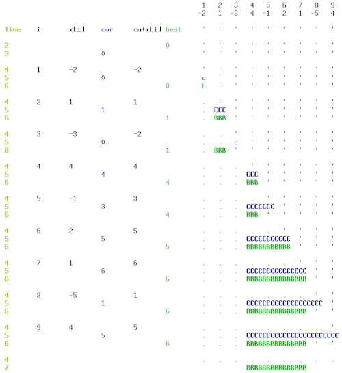
Execution of Kadane's algorithm on the above example array. Blue: subarray with largest sum ending at i; green: subarray with largest sum encountered so far; a lower case letter indicates an empty array; variable i is left implicit in Python code.

Kadane's algorithm scans the given array ${\displaystyle A[1\ldots n]}$ from left to right. In the ${\displaystyle j}$th step, it computes the subarray with the largest sum ending at ${\displaystyle j}$; this sum is maintained in variable current_sum.[note 3] Moreover, it computes the subarray with the largest sum anywhere in ${\displaystyle A[1\ldots j]}$, maintained in variable best_sum,[note 4] and easily obtained as the maximum of all values of current_sum seen so far, cf. line 7 of the algorithm.

As a loop invariant, in the ${\displaystyle j}$th step, the old value of current_sum holds the maximum over all ${\displaystyle i\in \{1,\ldots ,j\}}$ of the sum ${\displaystyle A[i]+\cdots +A[j-1]}$.[note 5] Therefore, current_sum${\displaystyle +A[j]}$[note 6] is the maximum over all ${\displaystyle i\in \{1,\ldots ,j\}}$ of the sum ${\displaystyle A[i]+\cdots +A[j]}$. To extend the latter maximum to cover also the case ${\displaystyle i=j+1}$, it is sufficient to consider also the empty subarray ${\displaystyle A[j+1\;\ldots \;j]}$. This is done in line 6 by assigning ${\displaystyle \max(0,}$current_sum${\displaystyle +A[j])}$ as the new value of current_sum, which after that holds the maximum over all ${\displaystyle i\in \{1,\ldots ,j+1\}}$ of the sum ${\displaystyle A[i]+\cdots +A[j]}$.

Thus, the problem can be solved with the following code,[4][7] expressed here in Python:

def max_subarray(numbers):
    """Find the largest sum of any contiguous subarray."""
    best_sum = 0  # or: float('-inf')
    current_sum = 0
    for x in numbers:
        current_sum = max(0, current_sum + x)
        best_sum = max(best_sum, current_sum)
    return best_sum

This version of the algorithm will return 0 if the input contains no positive elements (including when the input is empty). For the variant of the problem which disallows empty subarrays, best_sum should be initialized to negative infinity instead[11] and also in the for loop current_sum should be updated as max(x, current_sum + x).[note 7] In that case, if the input contains no positive element, the returned value is that of the largest element (i.e., the least negative value), or negative infinity if the input was empty.

The algorithm can be modified to keep track of the starting and ending indices of the maximum subarray as well:

def max_subarray(numbers):
    """Find a contiguous subarray with the largest sum."""
    best_sum = 0  # or: float('-inf')
    best_start = best_end = 0  # or: None
    current_sum = 0
    for current_end, x in enumerate(numbers):
        if current_sum <= 0:
            # Start a new sequence at the current element
            current_start = current_end
            current_sum = x
        else:
            # Extend the existing sequence with the current element
            current_sum += x

        if current_sum > best_sum:
            best_sum = current_sum
            best_start = current_start
            best_end = current_end + 1  # the +1 is to make 'best_end' exclusive

    return best_sum, best_start, best_end

In Python, arrays are indexed starting from 0, and the end index is typically excluded, so that the subarray [22, 33] in the array [-11, 22, 33, -44] would start at index 1 and end at index 3.

Because of the way this algorithm uses optimal substructures (the maximum subarray ending at each position is calculated in a simple way from a related but smaller and overlapping subproblem: the maximum subarray ending at the previous position) this algorithm can be viewed as a simple/trivial example of dynamic programming.

The runtime complexity of Kadane's algorithm is ${\displaystyle O(n)}$.[4][7]

Generalizations

Similar problems may be posed for higher-dimensional arrays, but their solutions are more complicated; see, e.g., Takaoka (2002). Brodal & Jørgensen (2007) showed how to find the k largest subarray sums in a one-dimensional array, in the optimal time bound ${\displaystyle O(n+k)}$.

The Maximum sum k-disjoint subarrays can also be computed in the optimal time bound ${\displaystyle O(n+k)}$ .[12]

See also

• Subset sum problem

Notes

1. By using a precomputed table of cumulative sums ${\displaystyle S[k]=\sum _{x=1}^{k}A[x]}$ to compute the subarray sum ${\displaystyle \sum _{x=i}^{j}A[x]=S[j]-S[i-1]}$ in constant time
2. since every algorithm must at least scan the array once which already takes O(n) time
3. named MaxEndingHere in Bentley (1989), and c in Gries (1982)
4. named MaxSoFar in Bentley (1989), and s in Gries (1982)
5. This sum is ${\displaystyle 0}$ when ${\displaystyle i=j}$, corresponding to the empty subarray ${\displaystyle A[j\ldots j-1]}$.
6. In the Python code, ${\displaystyle A[j]}$ is expressed as x, with the index ${\displaystyle j}$ left implicit.
7. While the latter modification is not mentioned by Bentley (1989), it achieves maintaining the modified loop invariant current_sum${\displaystyle =\max _{i\in \{1,...,j\}}A[i]+...+A[j]}$ at the beginning of the ${\displaystyle j}$th step.

References

1. Bentley 1989, p. 69.
2. Bentley 1989, p. 70.
3. Bentley 1989, p. 73.
4. Bentley 1989, p. 74.
5. Bentley 1984, p. 868-869.
6. Bentley 1989, p. 76-77.
7. Gries 1982, p. 211.
8. Gries 1982, p. 209-211.
9. Bird 1989, Sect.8, p.126.
10. Backurs, Dikkala & Tzamos 2016.
11. Bentley 1989, p. 78,171.
12. Bengtsson & Chen 2007.

• Backurs, Arturs; Dikkala, Nishanth; Tzamos, Christos (2016), "Tight Hardness Results for Maximum Weight Rectangles", Proc. 43rd International Colloquium on Automata, Languages, and Programming: 81:1–81:13, doi:10.4230/LIPIcs.ICALP.2016.81, S2CID 12720136
• Bae, Sung Eun (2007), Sequential and Parallel Algorithms for the Generalized Maximum Subarray Problem (PDF) (Ph.D. thesis), University of Canterbury, S2CID 2681670.
• Bengtsson, Fredrik; Chen, Jingsen (2007), Computing maximum-scoring segments optimally (PDF) (Research report), Luleå University of Technology
• Bentley, Jon (1984), "Programming Pearls: Algorithm Design Techniques", Communications of the ACM, 27 (9): 865–873, doi:10.1145/358234.381162, S2CID 207565329
• Bentley, Jon (May 1989), Programming Pearls (2nd? ed.), Reading, MA: Addison Wesley, ISBN 0-201-10331-1
• Bird, Richard S. (1989), "Algebraic Identities for Program Calculation" (PDF), The Computer Journal, 32 (2): 122–126, doi:10.1093/comjnl/32.2.122
• Brodal, Gerth Stølting; Jørgensen, Allan Grønlund (2007), "A linear time algorithm for the k maximal sums problem", Mathematical Foundations of Computer Science, Lecture Notes in Computer Science, 4708, Springer-Verlag, pp. 442–453, doi:10.1007/978-3-540-74456-6_40.
• Gries, David (1982), "A Note on the Standard Strategy for Developing Loop Invariants and Loops" (PDF), Science of Computer Programming, 2 (3): 207–241, doi:10.1016/0167-6423(83)90015-1, hdl:1813/6370
• Takaoka, Tadao (2002), "Efficient algorithms for the maximum subarray problem by distance matrix multiplication", Electronic Notes in Theoretical Computer Science, 61: 191–200, doi:10.1016/S1571-0661(04)00313-5.
• Tamaki, Hisao; Tokuyama, Takeshi (1998), "Algorithms for the Maximum Subarray Problem Based on Matrix Multiplication", Proceedings of the 9th Symposium on Discrete Algorithms (SODA): 446–452, retrieved November 17, 2018

External links

• TAN, Lirong. "Maximum Contiguous Subarray Sum Problems" (PDF). Archived from the original (PDF) on 2015-10-10. Retrieved 2017-10-26.
• Mu, Shin-Cheng (2010). "The Maximum Segment Sum Problem: Its Origin, and a Derivation".
• "Notes on Maximum Subarray Problem". 2012.
• www.algorithmist.com
• alexeigor.wikidot.com
• greatest subsequential sum problem on Rosetta Code
• geeksforgeeks page on Kadane's Algorithm