Pattern theory

Pattern theory, formulated by Ulf Grenander, is a mathematical formalism to describe knowledge of the world as patterns. It differs from other approaches to artificial intelligence in that it does not begin by prescribing algorithms and machinery to recognize and classify patterns; rather, it prescribes a vocabulary to articulate and recast the pattern concepts in precise language. Broad in its mathematical coverage, Pattern Theory spans algebra and statistics, as well as local topological and global entropic properties.

In addition to the new algebraic vocabulary, its statistical approach is novel in its aim to:

Identify the hidden variables of a data set using real world data rather than artificial stimuli, which was previously commonplace.
Formulate prior distributions for hidden variables and models for the observed variables that form the vertices of a Gibbs-like graph.
Study the randomness and variability of these graphs.
Create the basic classes of stochastic models applied by listing the deformations of the patterns.
Synthesize (sample) from the models, not just analyze signals with them.

The Brown University Pattern Theory Group was formed in 1972 by Ulf Grenander.[1] Many mathematicians are currently working in this group, noteworthy among them being the Fields Medalist David Mumford. Mumford regards Grenander as his "guru" in Pattern Theory.

Example: Natural Language Grammar

Grammar automaton

Grammar generators

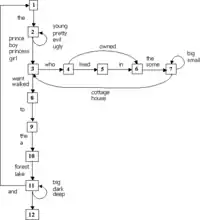
We begin with an example to motivate the algebraic definitions that follow. If we want to represent language patterns, the most immediate candidate for primitives might be words. However, set phrases, such as “in order to" immediately indicate the inappropriateness of words as atoms. In searching for other primitives, we might try the rules of grammar. We can represent grammars as finite state automata or context-free grammars. Below is a sample finite state grammar automaton.

The following phrases are generated from a few simple rules of the automaton and programming code in pattern theory:

the boy who owned the small cottage went to the deep forest

the prince walked to the lake

the girl walked to the lake and the princess went to the lake

the pretty prince walked to the dark forest

To create such sentences, rewriting rules in finite state automata act as generators to create the sentences as follows: if a machine starts in state 1, it goes to state 2 and writes the word “the”. From state 2, it writes one of 4 words: prince, boy, princess, girl, chosen at random. The probability of choosing any given word is given by the Markov chain corresponding to the automaton. Such a simplistic automaton occasionally generates more awkward sentences:

the evil evil prince walked to the lake

the prince walked to the dark forest and the prince walked to a forest and the princess who lived in some big small big cottage who owned the small big small house went to a forest

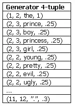
From the finite state diagram we can infer the following generators (shown at right) that creates the signal. A generator is a 4-tuple: current state, next state, word written, probability of written word when there are multiple choices. That is, each generator is a state transition arrow of state diagram for a Markov chain.

Imagine that a configuration of generators are strung together linearly so its output forms a sentence, so each generator "bonds" to the generators before and after it. Denote these bonds as 1x,1y,2x,2y,...12x,12y. Each numerical label corresponds to the automaton's state and each letter "x" and "y" corresponds to the inbound and outbound bonds. Then the following bond table (left) is equivalent to the automaton diagram. For the sake of simplicity, only half of the bond table is shown—the table is actually symmetric.

	1x	1y	2x	2y	3x	3y	4x	4y	5x	5y	6x	6y	7x	7y	8x	8y	9x	9y	10x	10y	11x	11y	12x	12y
1x	—	—	—	—	—	—	—	—	—	—	—	—	—	—	—	—	—	—	—	—	—	1	—	—
1y		—	1	—	—	—	—	—	—	—	—	—	—	—	—	—	—	—	—	—	—	—	—	—
2x			—	1	—	—	—	—	—	—	—	—	—	—	—	—	—	—	—	—	—	—	—	—
2y				—	1	—	—	—	—	—	—	—	—	—	—	—	—	—	—	—	—	—	—	—
3x					—	—	—	—	—	—	—	—	—	1	—	—	—	—	—	—	—	—	—	—
3y						—	1	—	—	—	—	—	—	—	1	—	—	—	—	—	—	—	—	—
4x							—	—	—	—	—	—	—	—	—	—	—	—	—	—	—	—	—	—
4y								—	1	—	1	—	—	—	—	—	—	—	—	—	—	—	—	—
5x									—	—	—	—	—	—	—	—	—	—	—	—	—	—	—	—
5y										—	1	—	—	—	—	—	—	—	—	—	—	—	—	—
6x											—	—	—	—	—	—	—	—	—	—	—	—	—	—
6y												—	1	—	—	—	—	—	—	—	—	—	—	—
7x													—	1	—	—	—	—	—	—	—	—	—	—
7y														—	—	—	—	—	—	—	—	—	—	—
8x															—	—	—	—	—	—	—	—	—	—
8y																—	1	—	—	—	—	—	—	—
9x																	—	—	—	—	—	—	—	—
9y																		—	1	—	—	—	—	—
10x																			—	—	—	—	—	—
10y																				—	1	—	—	—
11x																					—	1	—	—
11y																						—	1	—
12x																							—	—
12y																								—

As one can tell from this example, and typical of signals that are studied, identifying the primitives and bond tables requires some thought. The example highlights another important fact not readily apparent in other signals problems: that a configuration is not the signal that is observed; rather, its image as a sentence is observed. Herein lies a significant justification for distinguishing an observable from a non-observable construct. Additionally, it provides an algebraic structure to associate with hidden Markov models. In sensory examples such as the vision example below, the hidden configurations and observed images are much more similar, and such a distinction may not seem justified. Fortunately, the grammar example reminds us of this distinction.

A more sophisticated example can be found in the link grammar theory of natural language.

Algebraic foundations

Motivated by the example, we have the following definitions:

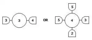
A generator $g{\in }G$ , drawn as

is the primitive of Pattern Theory that generates the observed signal. Structurally, it is a value with interfaces, called bonds $b{\in }B$ , which connects the $g$ 's to form a signal generator. 2 neighboring generators are connected when their bond values are the same. Similarity self-maps $s{\in }S$ s: G -> G express the invariances of the world we are looking at, such as rigid body transformations, or scaling.
Bonds glue generators into a configuration, c, which creates the signal against a backdrop Σ, with global features described locally by a bond coupling table called $\rho$ . The boolean function $\rho$ is the principal component of the regularity 4-tuple <G,S, ρ,Σ>, which is defined as
$\rho (c)=\prod _{{\text{neighboring bonds }}b',b''\in c}\rho (b',b'').$

$\rho$ seems to capture the notion of allowable generator neighbors. That is, Regularity is the law of the stimulus domain defining, via a bond table, what neighbors are acceptable for a generator. It is the laws of the stimulus domain. Later, we will relax regularity from a boolean function to a probability value, it would capture what stimulus neighbors are probable.

Σ is the physical arrangement of the generators. In vision, it could be a 2-dimensional lattice. In language, it is a linear arrangement.
An image (C mod R) captures the notion of an observed Configuration, as opposed to one which exists independently from any perceptual apparatus. Images are configurations distinguished only by their external bonds, inheriting the configuration's composition and similarities transformations. Formally, images are equivalence classes partitioned by an Identification Rule "~" with 3 properties:
1. ext(c) = ext(c') whenever c~c'
2. sc~sc' whenever c~c'
3. sigma(c1,c2) ~ sigma(c1',c2') whenever c1~c1', c2~c2' are all regular.
A configuration corresponding to a physical stimulus may have many images, corresponding to many observer perception's identification rule.
A pattern is the repeatable components of an image, defined as the S-invariant subset of an image. Similarities are reference transformations we use to define patterns, e.g. rigid body transformations. At first glance, this definition seems suited for only texture patterns where the minimal sub-image is repeated over and over again. If we were to view an image of an object such as a dog, it is not repeated, yet seem like it seems familiar and should be a pattern.
A deformation is a transformation of the original image that accounts for the noise in the environment and error in the perceptual apparatus. Grenander identifies 4 types of deformations: noise and blur, multi-scale superposition, domain warping, and interruptions.
Example 2 Directed boundary

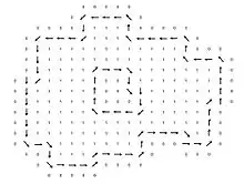Configuration

Image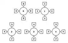

Generators

This configuration of generators generating the image is created by primitives woven together by the bonding table, and perceived by an observer with the identification rule that maps non "0" & "1" generators to a single boundary element. Nine other undepicted generators are created by rotating each of the non-"0"&"1" generators by 90 degrees. Keeping the feature of "directed boundaries" in mind, the generators are cooked with some thought and is interpreted as follows: the "0" generator corresponds to interior elements, "1" to the exterior, "2" and its rotations are straight elements, and the remainder are the turning elements.

With Boolean regularity defined as Product (all nbr bonds), any configurations with even a single generator violating the bond table is discarded from consideration. Thus only features in its purest form with all neighboring generators adhering to the bond table are allowed. This stringent condition can be relaxed using probability measures instead of Boolean bond tables.
$p(c)=\prod _{{\text{neighboring bonds }}b',b''\in c}A(b',b'')$

The new regularity no longer dictates a perfect directed boundary, but it defines a probability of a configuration in terms of the Acceptor function A(). Such configurations are allowed to have impurities and imperfections with respect to the feature of interest.

With the benefit of being given generators and complete bond tables, a difficult part of pattern analysis is done. In tackling a new class of signals and features, the task of devising the generators and bond table is much more difficult.

Again, just as in grammars, identifying the generators and bond tables require some thought. Just as subtle is the fact that a configuration is not the signal we observe. Rather, we observe its image as silhouette projections of the identification rule.

Boolean bonding truth table
Bond Values	0	1	2	3	4	5
0	1	—	—	—	1	—
1		1	—	—	—	1
2			—	1	—	—
3				—	—	—
4					—	—
5						—

Entropy

Pattern Theory defines order in terms of the feature of interest given by p(c).

Energy(c) = −log P(c)

Statistics

Grenander's Pattern Theory treatment of Bayesian inference in seems to be skewed towards on image reconstruction (e.g. content addressable memory). That is given image I-deformed, find I. However, Mumford's interpretation of Pattern Theory is broader and he defines PT to include many more well-known statistical methods. Mumford's criteria for inclusion of a topic as Pattern Theory are those methods "characterized by common techniques and motivations", such as the HMM, EM algorithm, dynamic programming circle of ideas. Topics in this section will reflect Mumford's treatment of Pattern Theory. His principle of statistical Pattern Theory are the following:

Use real world signals rather than constructed ones to infer the hidden states of interest.
Such signals contain too much complexity and artifacts to succumb to a purely deterministic analysis, so employ stochastic methods too.
Respect the natural structure of the signal, including any symmetries, independence of parts, marginals on key statistics. Validate by sampling from the derived models by and infer hidden states with Bayes’ rule.
Across all modalities, a limited family of deformations distort the pure patterns into real world signals.
Stochastic factors affecting an observation show strong conditional independence.

Statistical PT makes ubiquitous use of conditional probability in the form of Bayes theorem and Markov Models. Both these concepts are used to express the relation between hidden states (configurations) and observed states (images). Markov Models also captures the local properties of the stimulus, reminiscent of the purpose of bond table for regularity.

The generic set up is the following:

Let s = the hidden state of the data that we wish to know. i = observed image. Bayes theorem gives:

p (s | i ) p(i) = p (s, i ) = p (i|s ) p(s)

To analyze the signal (recognition): fix i, maximize p, infer s.

To synthesize signals (sampling): fix s, generate i's, compare w/ real world images

The following conditional probability examples illustrates these methods in action:

Conditional probability for local properties

N-gram Text Strings: See Mumford's Pattern Theory by Examples, Chapter 1.

MAP ~ MDL (MDL offers a glimpse of why the MAP probabilistic formulation make sense analytically)

Bayes Theorem for Machine translation

Supposing we want to translate French sentences to English. Here, the hidden configurations are English sentences and the observed signal they generate are French sentences. Bayes theorem gives p(e|f)p(f) = p(e, f) = p(f|e)p(e) and reduces to the fundamental equation of machine translation: maximize p(e|f) = p(f|e)p(e) over the appropriate e (note that p(f) is independent of e, and so drops out when we maximize over e). This reduces the problem to three main calculations for:

p(e) for any given e, using the N-gram method and dynamic programming
p(f|e) for any given e and f, using alignments and an expectation-maximization (EM) algorithm
e that maximizes the product of 1 and 2, again, using dynamic programming

The analysis seems to be symmetric with respect to the two languages, and if we think can calculate p(f|e), why not turn the analysis around and calculate p(e|f) directly? The reason is that during the calculation of p(f|e) the asymmetric assumption is made that source sentence be well formed and we cannot make any such assumption about the target translation because we do not know what it will translate into.

We now focus on p(f|e) in the three-part decomposition above. The other two parts, p(e) and maximizing e, uses similar techniques as the N-gram model. Given a French-English translation from a large training data set (such data sets exists from the Canadian parliament):

       NULL   And    the    program      has    been    implemented
                     Le     programme    a ete     mis en application

the sentence pair can be encoded as an alignment (2, 3, 4, 5, 6, 6, 6) that reads as follows: the first word in French comes from the second English word, the second word in French comes from the 3rd English word, and so forth. Although an alignment is a straightforward encoding of the translation, a more computationally convenient approach to an alignment is to break it down into four parameters:

Fertility: the number of words in the French string that will be connected to it. E.g. n( 3 | implemented ) = probability that “implemented” translates into three words – the word's fertility
Spuriousness: we introduce the artifact NULL as a word to represent the probability of tossing in a spurious French word. E.g. $p 1$ and its complement will be $p 0 = 1 - p 1$ .
Translation: the translated version of each word. E.g. t(a | has ) = translation probability that the English "has" translates into the French "a".
Distortion: the actual positions in the French string that these words will occupy. E.g. d( 5 | 2, 4, 6 ) = distortion of second position French word moving into the fifth position English word for a four-word English sentence and a six-word French sentence. We encode the alignments this way to easily represent and extract priors from our training data and the new formula becomes

{\begin{aligned}p(f|e)&={\text{Sum over all possible alignments an of }}p(a,f|e)\\&=n_{0}(v_{0}|\sum _{j=1}^{l}{v_{j}})\cdot \prod _{j=1}^{l}n(v_{j}|e_{j})v_{j}!\cdot \prod _{j=1}^{m}t(f_{j}|e_{a_{j}})\cdot \prod _{j:a_{j}\not =0}^{m}d(j|a_{j},l,m)\end{aligned}}

For the sake of simplicity in demonstrating an EM algorithm, we shall go through a simple calculation involving only translation probabilities t(), but needless to say that it the method applies to all parameters in their full glory. Consider the simplified case (1) without the NULL word (2) where every word has fertility 1 and (3) there are no distortion probabilities. Our training data corpus will contain two-sentence pairs: bc → xy and b → y. The translation of a two-word English sentence “b c” into the French sentence “x y” has two possible alignments, and including the one-sentence words, the alignments are:

                         b c   b c   b
                         | |    x    |
                         x y   x y   y

called Parallel, Crossed, and Singleton respectively.

To illustrate an EM algorithm, first set the desired parameter uniformly, that is

t(x | b ) = t(y | b ) = t(x | c ) = t(y | c ) = ¹⁄₂

Then EM iterates as follows

Iterations of an EM algorithm

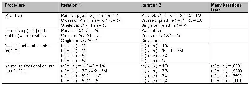
The alignment probability for the “crossing alignment” (where b connects to y) got a boost from the second sentence pair b/y. That further solidified t(y | b), but as a side effect also boosted t(x | c), because x connects to c in that same “crossing alignment.” The effect of boosting t(x | c) necessarily means downgrading t(y | c) because they sum to one. So, even though y and c co-occur, analysis reveals that they are not translations of each other. With real data, EM also is subject to the usual local extremum traps.

HMMs for speech recognition

Vibrational breakdown of "ski"

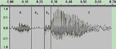
For decades, speech recognition seemed to hit an impasse as scientists sought descriptive and analytic solution. The sound wave p(t) below is produced by speaking the word “ski”.

Its four distinct segments has very different characteristics. One can choose from many levels of generators (hidden variables): the intention of the speaker's brain, the state of the mouth and vocal cords, or the ‘phones’ themselves. Phones are the generator of choice to be inferred and it encodes the word in a noisy, highly variable way. Early work on speech recognition attempted to make this inference deterministically using logical rules based on binary features extracted from p(t). For instance, the table below shows some of the features used to distinguish English consonants.

In real situations, the signal is further complicated by background noises such as cars driving by or artifacts such as a cough in mid sentence (Mumford's 2nd underpinning). The deterministic rule-based approach failed and the state of the art (e.g. Dragon NaturallySpeaking) is to use a family of precisely tuned HMMs and Bayesian MAP estimators to do better. Similar stories played out in vision, and other stimulus categories.

Deterministic approach to speech recognition
	p	t	k	b	d	g	m	n	f	s	v	z
Continuant	—	—	—	—	—	—	—	—	$+$	$+$	$+$	$+$
Voiced	—	—	—	$+$	$+$	$+$	$+$	$+$	—	—	$+$	$+$
Nasal	—	—	—	—	—	—	$+$	$+$	—	—	—	—
Labial	$+$	—	—	$+$	—	—	$+$	—	$+$	—	$+$	—
Coronal	—	$+$	—	—	$+$	—	—	$+$	—	$+$	—	$+$
Anterior	$+$	$+$	—	$+$	$+$	—	$+$	$+$	$+$	$+$	$+$	$+$
Strident	—	—	—	—	—	—	—	—	$+$	$+$	$+$	$+$

(See Mumford's Pattern Theory: the mathematics of perception)

The Markov stochastic process is diagrammed as follows:

\dots ,x_{k},x_{k+1},\dots \Pr(x,s)=\prod _{k}p_{1}(x_{k}|x_{k-1})p_{2}(s_{k}|x_{k})

exponentials, EM algorithm

References

"Ulf Grenander's Home Page". January 22, 2009. Archived from the original on 2009-01-22.

External links

Pattern Theory Group at Brown University
Pattern Theory: Grenander's Ideas and Examples - a video lecture by David Mumford
Pattern Theory and Applications - graduate course page with material by a Brown University alumnus

This article is issued from Wikipedia. The text is licensed under Creative Commons - Attribution - Sharealike. Additional terms may apply for the media files.

[1] "Ulf Grenander's Home Page". January 22, 2009. Archived from the original on 2009-01-22.