Hyperbolic geometric graph
A hyperbolic geometric graph (HGG) or hyperbolic geometric network (HGN) is a special type of spatial network where (1) latent coordinates of nodes are sprinkled according to a probability density function into a hyperbolic space of constant negative curvature and (2) an edge between two nodes is present if they are close according to a function of the metric[1][2] (typically either a Heaviside step function resulting in deterministic connections between vertices closer than a certain threshold distance, or a decaying function of hyperbolic distance yielding the connection probability). A HGG generalizes a random geometric graph (RGG) whose embedding space is Euclidean.
| Network science | ||||
|---|---|---|---|---|
| Network types | ||||
| Graphs | ||||
|
||||
| Models | ||||
|
||||
| ||||
|
||||
Mathematical formulation
Mathematically, a HGG is a graph with a vertex set V (cardinality ) and an edge set E constructed by considering the nodes as points placed onto a 2-dimensional hyperbolic space of constant negative Gaussian curvature, and cut-off radius , i.e. the radius of the Poincaré disk which can be visualized using a hyperboloid model. Each point has hyperbolic polar coordinates with and .
The hyperbolic law of cosines allows to measure the distance between two points and ,[2]
The angle is the (smallest) angle between the two position vectors.
In the simplest case, an edge is established iff (if and only if) two nodes are within a certain neighborhood radius , , this corresponds to an influence threshold.
Connectivity decay function
In general, a link will be established with a probability depending on the distance . A connectivity decay function represents the probability of assigning an edge to a pair of nodes at distance . In this framework, the simple case of hard-code neighborhood like in random geometric graphs is referred to as truncation decay function.[3]
Generating hyperbolic geometric graphs
Krioukov et al.[2] describe how to generate hyperbolic geometric graphs with uniformly random node distribution (as well as generalized versions) on a disk of radius in . These graphs yield a power-law distribution for the node degrees. The angular coordinate of each point/node is chosen uniformly random from , while the density function for the radial coordinate r is chosen according to the probability distribution :
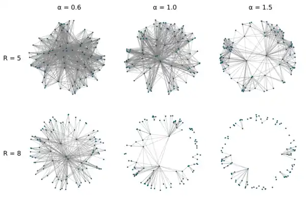
The growth parameter controls the distribution: For , the distribution is uniform in , for smaller values the nodes are distributed more towards the center of the disk and for bigger values more towards the border. In this model, edges between nodes and exist iff or with probability if a more general connectivity decay function is used. The average degree is controlled by the radius of the hyperbolic disk. It can be shown, that for the node degrees follow a power law distribution with exponent .
The image depicts randomly generated graphs for different values of and in . It can be seen how has an effect on the distribution of the nodes and on the connectivity of the graph. The native representation where the distance variables have their true hyperbolic values is used for the visualization of the graph, therefore edges are straight lines.

Quadratic complexity generator[4]
The naive algorithm for the generation of hyperbolic geometric graphs distributes the nodes on the hyperbolic disk by choosing the angular and radial coordinates of each point are sampled randomly. For every pair of nodes an edge is then inserted with the probability of the value of the connectivity decay function of their respective distance. The pseudocode looks as follows:
for to do for every pair do if then return
is the number of nodes to generate, the distribution of the radial coordinate by the probability density function is achieved by using inverse transform sampling. denotes the uniform sampling of a value in the given interval. Because the algorithm checks for edges for all pairs of nodes, the runtime is quadratic. For applications where is big, this is not viable any more and algorithms with subquadratic runtime are needed.
Sub-quadratic generation
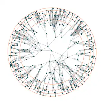
To avoid checking for edges between every pair of nodes, modern generators use additional data structures that partition the graph into bands.[5][6] A visualization of this shows a hyperbolic graph with the boundary of the bands drawn in orange. In this case, the partitioning is done along the radial axis. Points are stored sorted by their angular coordinate in their respective band. For each point , the limits of its hyperbolic circle of radius can be (over-)estimated and used to only perform the edge-check for points that lie in a band that intersects the circle. Additionally, the sorting within each band can be used to further reduce the number of points to look at by only considering points whose angular coordinate lie in a certain range around the one of (this range is also computed by over-estimating the hyperbolic circle around ).
Using this and other extensions of the algorithm, time complexities of (where is the number of nodes and the number of edges) are possible with high probability.[7]

Findings
For (Gaussian curvature ), HGGs form an ensemble of networks for which is possible to express the degree distribution analytically as closed form for the limiting case of large number of nodes.[2] This is worth mentioning since this is not true for many ensembles of graphs.
Applications
HGGs have been suggested as promising model for social networks where the hyperbolicity appears through a competition between similarity and popularity of an individual.[8]
References
- Barthélemy, Marc (2011). "Spatial networks". Physics Reports. 499 (1–3): 1–101. arXiv:1010.0302. Bibcode:2011PhR...499....1B. doi:10.1016/j.physrep.2010.11.002. S2CID 4627021.
- Krioukov, Dmitri; Papadopoulos, Fragkiskos; Kitsak, Maksim; Vahdat, Amin; Boguñá, Marián (2010). "Hyperbolic geometry of complex networks". Physical Review E. 82 (3): 036106. arXiv:1006.5169. Bibcode:2010PhRvE..82c6106K. doi:10.1103/PhysRevE.82.036106. PMID 21230138. S2CID 6451908.
- Barnett, L.; Di Paolo, E.; Bullock, S. (2007). "Spatially embedded random networks" (PDF). Physical Review E. 76 (5): 056115. Bibcode:2007PhRvE..76e6115B. doi:10.1103/PhysRevE.76.056115. PMID 18233726.
- Krioukov, Dmitri; Orsini, Chiara; Aldecoa, Rodrigo (2015-03-17). "Hyperbolic Graph Generator". Computer Physics Communications. 196: 492–496. arXiv:1503.05180. Bibcode:2015CoPhC.196..492A. doi:10.1016/j.cpc.2015.05.028. S2CID 8454036.
- von Looz, Moritz; Meyerhenke, Henning; Prutkin, Roman (2015). Elbassioni, Khaled; Makino, Kazuhisa (eds.). "Generating Random Hyperbolic Graphs in Subquadratic Time". Algorithms and Computation. Lecture Notes in Computer Science. Springer Berlin Heidelberg. 9472: 467–478. doi:10.1007/978-3-662-48971-0_40. ISBN 9783662489710.
- Meyerhenke, Henning; Laue, Sören; Özdayi, Mustafa; von Looz, Moritz (2016-06-30). "Generating massive complex networks with hyperbolic geometry faster in practice". arXiv:1606.09481. Bibcode:2016arXiv160609481V. Cite journal requires
|journal=(help) - Penschuck, Manuel (2017). "Generating Practical Random Hyperbolic Graphs in Near-Linear Time and with Sub-Linear Memory". Schloss Dagstuhl - Leibniz-Zentrum für Informatik GMBH, Wadern/Saarbruecken, Germany. Leibniz International Proceedings in Informatics (LIPIcs). 75: 26:1–26:21. doi:10.4230/lipics.sea.2017.26. ISBN 9783959770361.
- Papadopoulos, Fragkiskos; Kitsak, Maksim; Serrano, M. Ángeles; Boguñá, Marián; Krioukov, Dmitri (12 September 2012). "Popularity versus similarity in growing networks". Nature. 489 (7417): 537–540. arXiv:1106.0286. Bibcode:2012Natur.489..537P. doi:10.1038/nature11459. PMID 22972194. S2CID 4424179.
