Logistic function

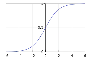
A logistic function or logistic curve is a common S-shaped curve (sigmoid curve) with equation

${\displaystyle f(x)={\frac {L}{1+e^{-k(x-x_{0})}}},}$

Standard logistic sigmoid function i.e. ${\displaystyle L=1,k=1,x_{0}=0}$

where

${\displaystyle x_{0}}$, the ${\displaystyle x}$ value of the sigmoid's midpoint;

${\displaystyle L}$, the curve's maximum value;

${\displaystyle k}$, the logistic growth rate or steepness of the curve.[1]

For values of ${\displaystyle x}$ in the domain of real numbers from ${\displaystyle -\infty }$ to ${\displaystyle +\infty }$, the S-curve shown on the right is obtained, with the graph of ${\displaystyle f}$ approaching ${\displaystyle L}$ as ${\displaystyle x}$ approaches ${\displaystyle +\infty }$ and approaching zero as ${\displaystyle x}$ approaches ${\displaystyle -\infty }$.

The logistic function finds applications in a range of fields, including biology (especially ecology), biomathematics, chemistry, demography, economics, geoscience, mathematical psychology, probability, sociology, political science, linguistics, statistics, and artificial neural networks. A generalization of the logistic function is the hyperbolastic function of type I.

History

Original image of a logistic curve, contrasted with a logarithmic curve

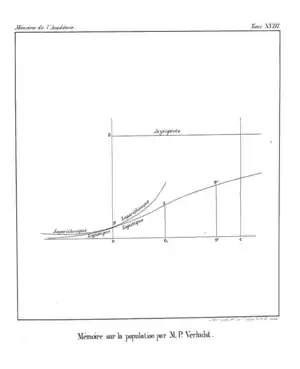
The logistic function was introduced in a series of three papers by Pierre François Verhulst between 1838 and 1847, who devised it as a model of population growth by adjusting the exponential growth model, under the guidance of Adolphe Quetelet.[2] Verhulst first devised the function in the mid 1830s, publishing a brief note in 1838,[1] then presented an expanded analysis and named the function in 1844 (published 1845);[lower-alpha 1][3] the third paper adjusted the correction term in his model of Belgian population growth.[4]

The initial stage of growth is approximately exponential (geometric); then, as saturation begins, the growth slows to linear (arithmetic), and at maturity, growth stops. Verhulst did not explain the choice of the term "logistic" (French: logistique), but it is presumably in contrast to the logarithmic curve,[5][lower-alpha 2] and by analogy with arithmetic and geometric. His growth model is preceded by a discussion of arithmetic growth and geometric growth (whose curve he calls a logarithmic curve, instead of the modern term exponential curve), and thus "logistic growth" is presumably named by analogy, logistic being from Ancient Greek: λογῐστῐκός, romanized: logistikós, a traditional division of Greek mathematics.[lower-alpha 3] The term is unrelated to the military and management term logistics, which is instead from French: logis "lodgings", though some believe the Greek term also influenced logistics; see Logistics § Origin for details.

Mathematical properties

The standard logistic function is the logistic function with parameters ${\displaystyle k=1}$, ${\displaystyle x_{0}=0}$, ${\displaystyle L=1}$, which yields

${\displaystyle f(x)={\frac {1}{1+e^{-x}}}={\frac {e^{x}}{e^{x}+1}}={\frac {1}{2}}+{\frac {1}{2}}\tanh \left({\frac {x}{2}}\right).}$

In practice, due to the nature of the exponential function ${\displaystyle e^{-x}}$, it is often sufficient to compute the standard logistic function for ${\displaystyle x}$ over a small range of real numbers, such as a range contained in [−6, +6], as it quickly converges very close to its saturation values of 0 and 1.

The logistic function has the symmetry property that

${\displaystyle 1-f(x)=f(-x).}$

Thus, ${\displaystyle x\mapsto f(x)-1/2}$ is an odd function.

The logistic function is an offset and scaled hyperbolic tangent function:

${\displaystyle f(x)={\frac {1}{2}}+{\frac {1}{2}}\tanh \left({\frac {x}{2}}\right),}$

or

${\displaystyle \tanh(x)=2f(2x)-1.}$

This follows from

${\displaystyle {\begin{aligned}\tanh(x)&={\frac {e^{x}-e^{-x}}{e^{x}+e^{-x}}}={\frac {e^{x}\cdot \left(1-e^{-2x}\right)}{e^{x}\cdot \left(1+e^{-2x}\right)}}\\&=f(2x)-{\frac {e^{-2x}}{1+e^{-2x}}}=f(2x)-{\frac {e^{-2x}+1-1}{1+e^{-2x}}}=2f(2x)-1.\end{aligned}}}$

Derivative

The standard logistic function has an easily calculated derivative. The derivative is known as the logistic distribution:

${\displaystyle f(x)={\frac {1}{1+e^{-x}}}={\frac {e^{x}}{1+e^{x}}},}$

${\displaystyle {\frac {\mathrm {d} }{\mathrm {d} x}}f(x)={\frac {e^{x}\cdot (1+e^{x})-e^{x}\cdot e^{x}}{(1+e^{x})^{2}}}={\frac {e^{x}}{(1+e^{x})^{2}}}=f(x){\big (}1-f(x){\big )}=f(x)f(-x).}$

The derivative of the logistic function is an even function, that is,

${\displaystyle f'(-x)=f'(x).}$

Integral

Conversely, its antiderivative can be computed by the substitution ${\displaystyle u=1+e^{x}}$, since ${\displaystyle f(x)={\frac {e^{x}}{1+e^{x}}}={\frac {u'}{u}}}$, so (dropping the constant of integration)

${\displaystyle \int {\frac {e^{x}}{1+e^{x}}}\,dx=\int {\frac {1}{u}}\,du=\ln u=\ln(1+e^{x}).}$

In artificial neural networks, this is known as the softplus function and (with scaling) is a smooth approximation of the ramp function, just as the logistic function (with scaling) is a smooth approximation of the Heaviside step function.

Logistic differential equation

The standard logistic function is the solution of the simple first-order non-linear ordinary differential equation

${\displaystyle {\frac {d}{dx}}f(x)=f(x){\big (}1-f(x){\big )}}$

with boundary condition ${\displaystyle f(0)=1/2}$. This equation is the continuous version of the logistic map. Note that the reciprocal logistic function is solution to a simple first-order linear ordinary differential equation.[6]

The qualitative behavior is easily understood in terms of the phase line: the derivative is 0 when the function is 1; and the derivative is positive for ${\displaystyle f}$ between 0 and 1, and negative for ${\displaystyle f}$ above 1 or less than 0 (though negative populations do not generally accord with a physical model). This yields an unstable equilibrium at 0 and a stable equilibrium at 1, and thus for any function value greater than 0 and less than 1, it grows to 1.

The logistic equation is a special case of the Bernoulli differential equation and has the following solution:

${\displaystyle f(x)={\frac {e^{x}}{e^{x}+C}}.}$

Choosing the constant of integration ${\displaystyle C=1}$ gives the other well known form of the definition of the logistic curve:

${\displaystyle f(x)={\frac {e^{x}}{e^{x}+1}}={\frac {1}{1+e^{-x}}}.}$

More quantitatively, as can be seen from the analytical solution, the logistic curve shows early exponential growth for negative argument, which slows to linear growth of slope 1/4 for an argument near 0, then approaches 1 with an exponentially decaying gap.

The logistic function is the inverse of the natural logit function and so can be used to convert the logarithm of odds into a probability. In mathematical notation the logistic function is sometimes written as expit[7] in the same form as logit. The conversion from the log-likelihood ratio of two alternatives also takes the form of a logistic curve.

The differential equation derived above is a special case of a general differential equation that only models the sigmoid function for ${\displaystyle x>0}$. In many modeling applications, the more general form[8]

${\displaystyle {\frac {df(x)}{dx}}={\frac {k}{a}}f(x){\big (}a-f(x){\big )},\quad f(0)=a/(1+e^{kr})}$

can be desirable. Its solution is the shifted and scaled sigmoid ${\displaystyle aS{\big (}k(x-r){\big )}}$.

The hyperbolic-tangent relationship leads to another form for the logistic function's derivative:

${\displaystyle {\frac {d}{dx}}f(x)={\frac {1}{4}}\operatorname {sech} ^{2}\left({\frac {x}{2}}\right),}$

which ties the logistic function into the logistic distribution.

Rotational symmetry about (0, 1/2)

The sum of the logistic function and its reflection about the vertical axis, ${\displaystyle f(-x)}$, is

${\displaystyle {\frac {1}{1+e^{-x}}}+{\frac {1}{1+e^{-(-x)}}}={\frac {e^{x}}{e^{x}+1}}+{\frac {1}{e^{x}+1}}=1.}$

The logistic function is thus rotationally symmetrical about the point (0, 1/2).[9]

Applications

Link[10] created an extension of Wald's theory of sequential analysis to a distribution-free accumulation of random variables until either a positive or negative bound is first equaled or exceeded. Link[11] derives the probability of first equaling or exceeding the positive boundary as ${\displaystyle (1+e^{-\theta A})}$, the Logistic function. This is the first proof that the Logistic function may have a stochastic process as its basis. Link[12] provides a century of examples of "Logistic" experimental results and a newly derived relation between this probability and the time of absorption at the boundaries.

In ecology: modeling population growth

Pierre-François Verhulst (1804–1849)

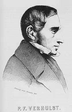
A typical application of the logistic equation is a common model of population growth (see also population dynamics), originally due to Pierre-François Verhulst in 1838, where the rate of reproduction is proportional to both the existing population and the amount of available resources, all else being equal. The Verhulst equation was published after Verhulst had read Thomas Malthus' An Essay on the Principle of Population, which describes the Malthusian growth model of simple (unconstrained) exponential growth. Verhulst derived his logistic equation to describe the self-limiting growth of a biological population. The equation was rediscovered in 1911 by A. G. McKendrick for the growth of bacteria in broth and experimentally tested using a technique for nonlinear parameter estimation.[13] The equation is also sometimes called the Verhulst-Pearl equation following its rediscovery in 1920 by Raymond Pearl (1879–1940) and Lowell Reed (1888–1966) of the Johns Hopkins University.[14] Another scientist, Alfred J. Lotka derived the equation again in 1925, calling it the law of population growth.

Letting ${\displaystyle P}$ represent population size (${\displaystyle N}$ is often used in ecology instead) and ${\displaystyle t}$ represent time, this model is formalized by the differential equation:

${\displaystyle {\frac {dP}{dt}}=rP\left(1-{\frac {P}{K}}\right),}$

where the constant ${\displaystyle r}$ defines the growth rate and ${\displaystyle K}$ is the carrying capacity.

In the equation, the early, unimpeded growth rate is modeled by the first term ${\displaystyle +rP}$. The value of the rate ${\displaystyle r}$ represents the proportional increase of the population ${\displaystyle P}$ in one unit of time. Later, as the population grows, the modulus of the second term (which multiplied out is ${\displaystyle -rP^{2}/K}$) becomes almost as large as the first, as some members of the population ${\displaystyle P}$ interfere with each other by competing for some critical resource, such as food or living space. This antagonistic effect is called the bottleneck, and is modeled by the value of the parameter ${\displaystyle K}$. The competition diminishes the combined growth rate, until the value of ${\displaystyle P}$ ceases to grow (this is called maturity of the population). The solution to the equation (with ${\displaystyle P_{0}}$ being the initial population) is

${\displaystyle P(t)={\frac {KP_{0}e^{rt}}{K+P_{0}\left(e^{rt}-1\right)}}={\frac {K}{1+\left({\frac {K-P_{0}}{P_{0}}}\right)e^{-rt}}},}$

where

${\displaystyle \lim _{t\to \infty }P(t)=K.}$

Which is to say that ${\displaystyle K}$ is the limiting value of ${\displaystyle P}$: the highest value that the population can reach given infinite time (or come close to reaching in finite time). It is important to stress that the carrying capacity is asymptotically reached independently of the initial value ${\displaystyle P(0)>0}$, and also in the case that ${\displaystyle P(0)>K}$.

In ecology, species are sometimes referred to as ${\displaystyle r}$-strategist or ${\displaystyle K}$-strategist depending upon the selective processes that have shaped their life history strategies. Choosing the variable dimensions so that ${\displaystyle n}$ measures the population in units of carrying capacity, and ${\displaystyle \tau }$ measures time in units of ${\displaystyle 1/r}$, gives the dimensionless differential equation

${\displaystyle {\frac {dn}{d\tau }}=n(1-n).}$

Time-varying carrying capacity

Since the environmental conditions influence the carrying capacity, as a consequence it can be time-varying, with ${\displaystyle K(t)>0}$, leading to the following mathematical model:

${\displaystyle {\frac {dP}{dt}}=rP\cdot \left(1-{\frac {P}{K(t)}}\right).}$

A particularly important case is that of carrying capacity that varies periodically with period ${\displaystyle T}$:

${\displaystyle K(t+T)=K(t).}$

It can be shown that in such a case, independently from the initial value ${\displaystyle P(0)>0}$, ${\displaystyle P(t)}$ will tend to a unique periodic solution ${\displaystyle P_{*}(t)}$, whose period is ${\displaystyle T}$.

A typical value of ${\displaystyle T}$ is one year: In such case ${\displaystyle K(t)}$ may reflect periodical variations of weather conditions.

Another interesting generalization is to consider that the carrying capacity ${\displaystyle K(t)}$ is a function of the population at an earlier time, capturing a delay in the way population modifies its environment. This leads to a logistic delay equation,[15] which has a very rich behavior, with bistability in some parameter range, as well as a monotonic decay to zero, smooth exponential growth, punctuated unlimited growth (i.e., multiple S-shapes), punctuated growth or alternation to a stationary level, oscillatory approach to a stationary level, sustainable oscillations, finite-time singularities as well as finite-time death.

In statistics and machine learning

Logistic functions are used in several roles in statistics. For example, they are the cumulative distribution function of the logistic family of distributions, and they are, a bit simplified, used to model the chance a chess player has to beat his opponent in the Elo rating system. More specific examples now follow.

Logistic regression

Logistic functions are used in logistic regression to model how the probability ${\displaystyle p}$ of an event may be affected by one or more explanatory variables: an example would be to have the model

${\displaystyle p=f(a+bx),}$

where ${\displaystyle x}$ is the explanatory variable, ${\displaystyle a}$ and ${\displaystyle b}$ are model parameters to be fitted, and ${\displaystyle f}$ is the standard logistic function.

Logistic regression and other log-linear models are also commonly used in machine learning. A generalisation of the logistic function to multiple inputs is the softmax activation function, used in multinomial logistic regression.

Another application of the logistic function is in the Rasch model, used in item response theory. In particular, the Rasch model forms a basis for maximum likelihood estimation of the locations of objects or persons on a continuum, based on collections of categorical data, for example the abilities of persons on a continuum based on responses that have been categorized as correct and incorrect.

Neural networks

Logistic functions are often used in neural networks to introduce nonlinearity in the model or to clamp signals to within a specified interval. A popular neural net element computes a linear combination of its input signals, and applies a bounded logistic function as the activation function to the result; this model can be seen as a "smoothed" variant of the classical threshold neuron.

A common choice for the activation or "squashing" functions, used to clip for large magnitudes to keep the response of the neural network bounded[16] is

${\displaystyle g(h)={\frac {1}{1+e^{-2\beta h}}},}$

which is a logistic function.

These relationships result in simplified implementations of artificial neural networks with artificial neurons. Practitioners caution that sigmoidal functions which are antisymmetric about the origin (e.g. the hyperbolic tangent) lead to faster convergence when training networks with backpropagation.[17]

The logistic function is itself the derivative of another proposed activation function, the softplus.

In medicine: modeling of growth of tumors

Another application of logistic curve is in medicine, where the logistic differential equation is used to model the growth of tumors. This application can be considered an extension of the above-mentioned use in the framework of ecology (see also the Generalized logistic curve, allowing for more parameters). Denoting with ${\displaystyle X(t)}$ the size of the tumor at time ${\displaystyle t}$, its dynamics are governed by

${\displaystyle X'=r\left(1-{\frac {X}{K}}\right)X,}$

which is of the type

${\displaystyle X'=F(X)X,\quad F'(X)\leq 0,}$

where ${\displaystyle F(X)}$ is the proliferation rate of the tumor.

If a chemotherapy is started with a log-kill effect, the equation may be revised to be

${\displaystyle X'=r\left(1-{\frac {X}{K}}\right)X-c(t)X,}$

where ${\displaystyle c(t)}$ is the therapy-induced death rate. In the idealized case of very long therapy, ${\displaystyle c(t)}$ can be modeled as a periodic function (of period ${\displaystyle T}$) or (in case of continuous infusion therapy) as a constant function, and one has that

${\displaystyle {\frac {1}{T}}\int _{0}^{T}c(t)\,dt>r\to \lim _{t\to +\infty }x(t)=0,}$

i.e. if the average therapy-induced death rate is greater than the baseline proliferation rate, then there is the eradication of the disease. Of course, this is an oversimplified model of both the growth and the therapy (e.g. it does not take into account the phenomenon of clonal resistance).

In medicine: modeling of a pandemic

A novel infectious pathogen to which a population has no immunity will generally spread exponentially in the early stages, while the supply of susceptible individuals is plentiful. The SARS-CoV-2 virus that causes COVID-19 exhibited exponential growth early in the course of infection in several countries in early 2020.[18] Many factors, ranging from lack of susceptibles (either through the continued spread of infection until it passes the threshold for herd immunity or reduction in the accessibility of susceptibles through physical distancing measures), exponential-looking epidemic curves may first linearize (replicating the "logarithmic" to "logistic" transition first noted by Pierre-François Verhulst, as noted above) and then reach a maximal limit.[19]

A logistic function, or related functions (e.g. the Gompertz function) are usually used in a descriptive or phenomenological manner because they fit well not only to the early exponential rise, but to the eventual levelling off of the pandemic as the population develops a herd immunity. This is in contrast to actual models of pandemics which attempt to formulate a description based on the dynamics of the pandemic (e.g. contact rates, incubation times, social distancing, etc.). Some simple models have been developed, however, which yield a logistic solution.[20][21][22]

Generalized logistic function (Richards growth curve) in epidemiological modeling

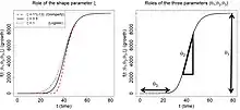
A generalized logistic function, also called the Richards growth curve, is widely used in modelling COVID-19 infection trajectories.[23] Infection trajectory is a daily time series data for the cumulative number of infected cases for a subject such as country, city, state, etc. There are variant re-parameterizations in the literature: one of frequently used forms is

${\displaystyle f(t;\theta _{1},\theta _{2},\theta _{3},\xi )={\frac {\theta _{1}}{[1+\xi \exp(-\theta _{2}\cdot (t-\theta _{3}))]^{1/\xi }}}}$

where ${\displaystyle \theta _{1},\theta _{2},\theta _{3}}$ are real numbers, and ${\displaystyle \xi }$ is a positive real number. The flexibility of the curve ${\displaystyle f}$ is due to the parameter ${\displaystyle \xi }$: (i) if ${\displaystyle \xi =1}$ then the curve reduces to the logistic function, and (ii) if ${\displaystyle \xi }$ converges to zero, then the curve converges to the Gompertz function. In epidemiological modeling, ${\displaystyle \theta _{1}}$, ${\displaystyle \theta _{2}}$, and ${\displaystyle \theta _{3}}$ represent the final epidemic size, infection rate, and lag phase, respectively. See the right panel for an examplary infection trajectory when ${\displaystyle (\theta _{1},\theta _{2},\theta _{3})}$ are designated by ${\displaystyle (10,000,0.2,40)}$.

One of the benefits of using growth function such as generalized logistic function in epidemiological modeling is its relatively easy expansion to the multilevel model framework by using the growth function to describe infection trajectories from multiple subjects (countries, cities, states, etc). Such a modeling framework can be also widely called the nonlinear mixed effect model or hierarchical nonlinear model. An example of using the generalized logistic function in Bayesian multilevel model is the Bayesian hierarchical Richards model.

In chemistry: reaction models

The concentration of reactants and products in autocatalytic reactions follow the logistic function. The degradation of Platinum group metal-free (PGM-free) oxygen reduction reaction (ORR) catalyst in fuel cell cathodes follows the logistic decay function,[24] suggesting an autocatalytic degradation mechanism.

In physics: Fermi–Dirac distribution

The logistic function determines the statistical distribution of fermions over the energy states of a system in thermal equilibrium. In particular, it is the distribution of the probabilities that each possible energy level is occupied by a fermion, according to Fermi–Dirac statistics.

In material science: Phase diagrams

See Diffusion bonding.

In linguistics: language change

In linguistics, the logistic function can be used to model language change:[25] an innovation that is at first marginal begins to spread more quickly with time, and then more slowly as it becomes more universally adopted.

In agriculture: modeling crop response

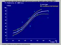
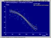
The logistic S-curve can be used for modeling the crop response to changes in growth factors. There are two types of response functions: positive and negative growth curves. For example, the crop yield may increase with increasing value of the growth factor up to a certain level (positive function), or it may decrease with increasing growth factor values (negative function owing to a negative growth factor), which situation requires an inverted S-curve.

S-curve model for crop yield versus depth of water table.[26]

Inverted S-curve model for crop yield versus soil salinity.[27]

In economics and sociology: diffusion of innovations

The logistic function can be used to illustrate the progress of the diffusion of an innovation through its life cycle.

In The Laws of Imitation (1890), Gabriel Tarde describes the rise and spread of new ideas through imitative chains. In particular, Tarde identifies three main stages through which innovations spread: the first one corresponds to the difficult beginnings, during which the idea has to struggle within a hostile environment full of opposing habits and beliefs; the second one corresponds to the properly exponential take-off of the idea, with ${\displaystyle f(x)=2^{x}}$; finally, the third stage is logarithmic, with ${\displaystyle f(x)=\log(x)}$, and corresponds to the time when the impulse of the idea gradually slows down while, simultaneously new opponent ideas appear. The ensuing situation halts or stabilizes the progress of the innovation, which approaches an asymptote.

In a Sovereign state, the subnational units (Constituent states or cities) may use loans to finance their projects. However, this funding source is usually subject to strict legal rules as well as to economy scarcity constraints, specially the resources the banks can lend (due to their equity or Basel limits). These restrictions, which represent a saturation level, along with an exponential rush in an economic competition for money, create a public finance diffusion of credit pleas and the aggregate national response is a sigmoid curve.[28]

In the history of economy, when new products are introduced there is an intense amount of research and development which leads to dramatic improvements in quality and reductions in cost. This leads to a period of rapid industry growth. Some of the more famous examples are: railroads, incandescent light bulbs, electrification, cars and air travel. Eventually, dramatic improvement and cost reduction opportunities are exhausted, the product or process are in widespread use with few remaining potential new customers, and markets become saturated.

Logistic analysis was used in papers by several researchers at the International Institute of Applied Systems Analysis (IIASA). These papers deal with the diffusion of various innovations, infrastructures and energy source substitutions and the role of work in the economy as well as with the long economic cycle. Long economic cycles were investigated by Robert Ayres (1989).[29] Cesare Marchetti published on long economic cycles and on diffusion of innovations.[30][31] Arnulf Grübler's book (1990) gives a detailed account of the diffusion of infrastructures including canals, railroads, highways and airlines, showing that their diffusion followed logistic shaped curves.[32]

Carlota Perez used a logistic curve to illustrate the long (Kondratiev) business cycle with the following labels: beginning of a technological era as irruption, the ascent as frenzy, the rapid build out as synergy and the completion as maturity.[33]

See also

• Exponential growth
• Hyperbolic growth
• Diffusion of innovations
• Generalised logistic function
• Gompertz curve
• Heaviside step function
• Hubbert curve
• Logistic distribution
• Logistic map
• Logistic regression
• Logistic smooth-transmission model
• Logit
• Log-likelihood ratio
• Malthusian growth model
• Population dynamics
• r/K selection theory
• Shifted Gompertz distribution
• Tipping point (sociology)
• Rectifier (neural networks)
• Cross fluid
• Hill equation (biochemistry)
• Michaelis–Menten equation

Notes

1. The paper was presented in 1844, and published in 1845: "(Lu à la séance du 30 novembre 1844)." "(Read at the session of 30 November 1844).", p. 1.
2. Verhulst first refers to arithmetic progression and geometric progression, and refers to the geometric growth curve as a logarithmic curve (confusingly, the modern term is instead exponential curve, which is the inverse). He then calls his curve logistic, in contrast to logarithmic, and compares the logarithmic curve and logistic curve in the figure of his paper.
3. In Ancient Greece, λογῐστῐκός referred to practical computation and accounting, in contrast to ἀριθμητική (arithmētikḗ), the theoretical or philosophical study of numbers. Confusingly, in English, arithmetic refers to practical computation, even though it derives from ἀριθμητική, not λογῐστῐκός. See for example Louis Charles Karpinski, Nicomachus of Gerasa: Introduction to Arithmetic (1926) p. 3: "Arithmetic is fundamentally associated by modern readers, particularly by scientists and mathematicians, with the art of computation. For the ancient Greeks after Pythagoras, however, arithmetic was primarily a philosophical study, having no necessary connection with practical affairs. Indeed the Greeks gave a separate name to the arithmetic of business, λογιστική [accounting or practical logistic] ... In general the philosophers and mathematicians of Greece undoubtedly considered it beneath their dignity to treat of this branch, which probably formed a part of the elementary instruction of children."

References

1. Verhulst, Pierre-François (1838). "Notice sur la loi que la population poursuit dans son accroissement" (PDF). Correspondance Mathématique et Physique. 10: 113–121. Retrieved 3 December 2014.
2. Cramer 2002, pp. 3–5.
3. Verhulst, Pierre-François (1845). "Recherches mathématiques sur la loi d'accroissement de la population" [Mathematical Researches into the Law of Population Growth Increase]. Nouveaux Mémoires de l'Académie Royale des Sciences et Belles-Lettres de Bruxelles. 18: 8. Retrieved 18 February 2013. Nous donnerons le nom de logistique à la courbe [We will give the name logistic to the curve]
4. Verhulst, Pierre-François (1847). "Deuxième mémoire sur la loi d'accroissement de la population". Mémoires de l'Académie Royale des Sciences, des Lettres et des Beaux-Arts de Belgique. 20: 1–32. Retrieved 18 February 2013.
5. Shulman, Bonnie (1998). "Math-alive! using original sources to teach mathematics in social context". PRIMUS. 8 (March): 1–14. doi:10.1080/10511979808965879. The diagram clinched it for me: there two curves labeled "Logistique" and "Logarithmique" are drawn on the same axes, and one can see that there is a region where they match almost exactly, and then diverge.
   I concluded that Verhulst's intention in naming the curve was indeed to suggest this comparison, and that "logistic" was meant to convey the curve's "log-like" quality.
6. Kocian, Alexander; Carmassi, Giulia; Cela, Fatjon; Incrocci, Luca; Milazzo, Paolo; Chessa, Stefano (7 June 2020). "Bayesian Sigmoid-Type Time Series Forecasting with Missing Data for Greenhouse Crops". Sensors. 20 (11): 3246. doi:10.3390/s20113246. PMC 7309099. PMID 32517314.
7. expit documentation for R's clusterPower package.
8. Kyurkchiev, Nikolay, and Svetoslav Markov. "Sigmoid functions: some approximation and modelling aspects". LAP LAMBERT Academic Publishing, Saarbrucken (2015).
9. Raul Rojas. Neural Networks – A Systematic Introduction (PDF). Retrieved 15 October 2016.
10. S. W. Link, Psychometrika, 1975, 40, 1, 77–105
11. S. W. Link, Attention and Performance VII, 1978, 619–630
12. S. W. Link, The wave theory of difference and similarity (book), Taylor and Francis, 1992
13. A. G. McKendricka; M. Kesava Paia1 (January 1912). "XLV.—The Rate of Multiplication of Micro-organisms: A Mathematical Study". Proceedings of the Royal Society of Edinburgh. 31: 649–653. doi:10.1017/S0370164600025426.
14. Raymond Pearl & Lowell Reed (June 1920). "On the Rate of Growth of the Population of the United States" (PDF). Proceedings of the National Academy of Sciences of the United States of America. 6 (6). p. 275.
15. Yukalov, V. I.; Yukalova, E. P.; Sornette, D. (2009). "Punctuated evolution due to delayed carrying capacity". Physica D: Nonlinear Phenomena. 238 (17): 1752–1767. arXiv:0901.4714. Bibcode:2009PhyD..238.1752Y. doi:10.1016/j.physd.2009.05.011. S2CID 14456352.
16. Gershenfeld 1999, p. 150.
17. LeCun, Y.; Bottou, L.; Orr, G.; Muller, K. (1998). Orr, G.; Muller, K. (eds.). Efficient BackProp (PDF). Neural Networks: Tricks of the trade. Springer. ISBN 3-540-65311-2.
18. Worldometer: COVID-19 CORONAVIRUS PANDEMIC
19. Villalobos-Arias, Mario (2020). "Using generalized logistics regression to forecast population infected by Covid-19". arXiv:2004.02406 [q-bio.PE].
20. Postnikov, Eugene B. (June 2020). "Estimation of COVID-19 dynamics "on a back-of-envelope": Does the simplest SIR model provide quantitative parameters and predictions?". Chaos, Solitons & Fractals. 135: 109841. doi:10.1016/j.chaos.2020.109841. PMC 7252058. PMID 32501369. Retrieved 20 July 2020.
21. Saito, Takesi (June 2020). "A Logistic Curve in the SIR Model and Its Application to Deaths by COVID-19 in Japan". MedRxiv. doi:10.1101/2020.06.25.20139865. S2CID 220068969. Retrieved 20 July 2020.
22. Reiser, Paul A. (2020). "Modified SIR Model Yielding a Logistic Solution". arXiv:2006.01550 [q-bio.PE].
23. Lee, Se Yoon; Lei, Bowen; Mallick, Bani (2020). "Estimation of COVID-19 spread curves integrating global data and borrowing information". PLOS ONE. 15 (7): e0236860. arXiv:2005.00662. Bibcode:2020PLoSO..1536860L. doi:10.1371/journal.pone.0236860. PMC 7390340. PMID 32726361.
24. Yin, Xi; Zelenay, Piotr (13 July 2018). "Kinetic Models for the Degradation Mechanisms of PGM-Free ORR Catalysts". ECS Transactions. 85 (13): 1239–1250. doi:10.1149/08513.1239ecst. OSTI 1471365.
25. Bod, Hay, Jennedy (eds.) 2003, pp. 147–156
26. Collection of data on crop production and depth of the water table in the soil of various authors. On line:
27. Collection of data on crop production and soil salinity of various authors. On line:
28. Rocha, Leno S.; Rocha, Frederico S. A.; Souza, Thársis T. P. (5 October 2017). "Is the public sector of your country a diffusion borrower? Empirical evidence from Brazil". PLOS ONE. 12 (10): e0185257. arXiv:1604.07782. Bibcode:2017PLoSO..1285257R. doi:10.1371/journal.pone.0185257. ISSN 1932-6203. PMC 5628819. PMID 28981532.
29. Ayres, Robert (1989). "Technological Transformations and Long Waves" (PDF). Cite journal requires |journal= (help)
30. Marchetti, Cesare (1996). "Pervasive Long Waves: Is Society Cyclotymic" (PDF). Archived from the original (PDF) on 5 March 2012. Cite journal requires |journal= (help)
31. Marchetti, Cesare (1988). "Kondratiev Revisited-After One Cycle" (PDF). Cite journal requires |journal= (help)
32. Grübler, Arnulf (1990). The Rise and Fall of Infrastructures: Dynamics of Evolution and Technological Change in Transport (PDF). Heidelberg and New York: Physica-Verlag.
33. Perez, Carlota (2002). Technological Revolutions and Financial Capital: The Dynamics of Bubbles and Golden Ages. UK: Edward Elgar Publishing Limited. ISBN 1-84376-331-1.

• Cramer, J. S. (2002). The origins of logistic regression (PDF) (Technical report). 119. Tinbergen Institute. pp. 167–178. doi:10.2139/ssrn.360300.
  • Published as:Cramer, J. S. (2004). "The early origins of the logit model". Studies in History and Philosophy of Science Part C: Studies in History and Philosophy of Biological and Biomedical Sciences. 35 (4): 613–626. doi:10.1016/j.shpsc.2004.09.003.
• Jannedy, Stefanie; Bod, Rens; Hay, Jennifer (2003). Probabilistic Linguistics. Cambridge, Massachusetts: MIT Press. ISBN 0-262-52338-8.
• Gershenfeld, Neil A. (1999). The Nature of Mathematical Modeling. Cambridge, UK: Cambridge University Press. ISBN 978-0-521-57095-4.
• Kingsland, Sharon E. (1995). Modeling nature: episodes in the history of population ecology. Chicago: University of Chicago Press. ISBN 0-226-43728-0.
• Weisstein, Eric W. "Logistic Equation". MathWorld.

External links

• L.J. Linacre, Why logistic ogive and not autocatalytic curve?, accessed 2009-09-12.
• https://web.archive.org/web/20060914155939/http://luna.cas.usf.edu/~mbrannic/files/regression/Logistic.html
• Weisstein, Eric W. "Sigmoid Function". MathWorld.
• Online experiments with JSXGraph
• Esses are everywhere.
• Seeing the s-curve is everything.
• Restricted Logarithmic Growth with Injection