Bias–variance tradeoff

In statistics and machine learning, the bias–variance tradeoff is the property of a model that the variance of the parameter estimates across samples can be reduced by increasing the bias in the estimated parameters. The bias–variance dilemma or bias–variance problem is the conflict in trying to simultaneously minimize these two sources of error that prevent supervised learning algorithms from generalizing beyond their training set:[1][2]

• The bias error is an error from erroneous assumptions in the learning algorithm. High bias can cause an algorithm to miss the relevant relations between features and target outputs (underfitting).
• The variance is an error from sensitivity to small fluctuations in the training set. High variance can cause an algorithm to model the random noise in the training data, rather than the intended outputs (overfitting).

Function and noisy data.

spread=5

spread=1

spread=0.1

A function (red) is approximated using radial basis functions (blue). Several trials are shown in each graph. For each trial, a few noisy data points are provided as a training set (top). For a wide spread (image 2) the bias is high: the RBFs cannot fully approximate the function (especially the central dip), but the variance between different trials is low. As spread decreases (image 3 and 4) the bias decreases: the blue curves more closely approximate the red. However, depending on the noise in different trials the variance between trials increases. In the lowermost image the approximated values for x=0 varies wildly depending on where the data points were located.

The bias–variance decomposition is a way of analyzing a learning algorithm's expected generalization error with respect to a particular problem as a sum of three terms, the bias, variance, and a quantity called the irreducible error, resulting from noise in the problem itself.

Motivation

The bias-variance tradeoff is a central problem in supervised learning. Ideally, one wants to choose a model that both accurately captures the regularities in its training data, but also generalizes well to unseen data. Unfortunately, it is typically impossible to do both simultaneously. High-variance learning methods may be able to represent their training set well but are at risk of overfitting to noisy or unrepresentative training data. In contrast, algorithms with high bias typically produce simpler models that don't tend to overfit but may underfit their training data, failing to capture important regularities.

It is an often made fallacy[3][4] to assume that complex models must have high variance; High variance models are 'complex' in some sense, but the reverse needs not be true. In addition one has to be careful how to define complexity: In particular, the number of parameters used to describe the model is a poor measure of complexity. This is illustrated by an example adapted from:[5] The model ${\displaystyle f_{a,b}(x)=a\sin(bx)}$ has only two parameters (${\displaystyle a,b}$) but it can interpolate any number of points by oscillating with a high enough frequency, resulting in both a high bias and high variance.

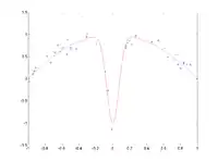
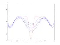
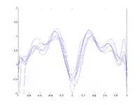
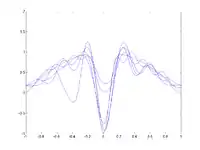
Intuitively, bias is reduced by using only local information, whereas variance can only be reduced by averaging over multiple observations, which inherently means using information from a larger region. For an enlightening example, see the section on k-nearest neighbors or the figure on the right. To balance how much information is used from neighboring observations, a model can be smoothed via explicit regularization, such as shrinkage.

Bias–variance decomposition of mean squared error

Suppose that we have a training set consisting of a set of points ${\displaystyle x_{1},\dots ,x_{n}}$ and real values ${\displaystyle y_{i}}$ associated with each point ${\displaystyle x_{i}}$. We assume that there is a function with noise ${\displaystyle y=f(x)+\varepsilon }$, where the noise, ${\displaystyle \varepsilon }$, has zero mean and variance ${\displaystyle \sigma ^{2}}$.

We want to find a function ${\displaystyle {\hat {f}}(x;D)}$, that approximates the true function ${\displaystyle f(x)}$ as well as possible, by means of some learning algorithm based on a training dataset (sample) ${\displaystyle D=\{(x_{1},y_{1})\dots ,(x_{n},y_{n})\}}$. We make "as well as possible" precise by measuring the mean squared error between ${\displaystyle y}$ and ${\displaystyle {\hat {f}}(x;D)}$: we want ${\displaystyle (y-{\hat {f}}(x;D))^{2}}$ to be minimal, both for ${\displaystyle x_{1},\dots ,x_{n}}$ and for points outside of our sample. Of course, we cannot hope to do so perfectly, since the ${\displaystyle y_{i}}$ contain noise ${\displaystyle \varepsilon }$; this means we must be prepared to accept an irreducible error in any function we come up with.

Finding an ${\displaystyle {\hat {f}}}$ that generalizes to points outside of the training set can be done with any of the countless algorithms used for supervised learning. It turns out that whichever function ${\displaystyle {\hat {f}}}$ we select, we can decompose its expected error on an unseen sample ${\displaystyle x}$ as follows:[6]^:34[7]^:223

${\displaystyle \operatorname {E} _{D}{\Big [}{\big (}y-{\hat {f}}(x;D){\big )}^{2}{\Big ]}={\Big (}\operatorname {Bias} _{D}{\big [}{\hat {f}}(x;D){\big ]}{\Big )}^{2}+\operatorname {Var} _{D}{\big [}{\hat {f}}(x;D){\big ]}+\sigma ^{2}}$

where

${\displaystyle \operatorname {Bias} _{D}{\big [}{\hat {f}}(x;D){\big ]}=\operatorname {E} _{D}{\big [}{\hat {f}}(x;D){\big ]}-f(x)}$

and

${\displaystyle \operatorname {Var} _{D}{\big [}{\hat {f}}(x;D){\big ]}=\operatorname {E} _{D}[{\big (}\operatorname {E} _{D}[{\hat {f}}(x;D)]-{\hat {f}}(x;D){\big )}^{2}].}$

The expectation ranges over different choices of the training set ${\displaystyle D=\{(x_{1},y_{1})\dots ,(x_{n},y_{n})\}}$, all sampled from the same joint distribution ${\displaystyle P(x,y)}$. The three terms represent:

• the square of the bias of the learning method, which can be thought of as the error caused by the simplifying assumptions built into the method. E.g., when approximating a non-linear function ${\displaystyle f(x)}$ using a learning method for linear models, there will be error in the estimates ${\displaystyle {\hat {f}}(x)}$ due to this assumption;
• the variance of the learning method, or, intuitively, how much the learning method ${\displaystyle {\hat {f}}(x)}$ will move around its mean;
• the irreducible error ${\displaystyle \sigma ^{2}}$.

Since all three terms are non-negative, this forms a lower bound on the expected error on unseen samples.[6]^:34

The more complex the model ${\displaystyle {\hat {f}}(x)}$ is, the more data points it will capture, and the lower the bias will be. However, complexity will make the model "move" more to capture the data points, and hence its variance will be larger.

Derivation

The derivation of the bias–variance decomposition for squared error proceeds as follows.[8][9] For notational convenience, we abbreviate ${\displaystyle f=f(x)}$, ${\displaystyle {\hat {f}}={\hat {f}}(x;D)}$ and we drop the ${\displaystyle D}$ subscript on our expectation operators. First, recall that, by definition, for any random variable ${\displaystyle X}$, we have

${\displaystyle \operatorname {Var} [X]=\operatorname {E} [X^{2}]-\operatorname {E} [X]^{2}.}$

Rearranging, we get:

${\displaystyle \operatorname {E} [X^{2}]=\operatorname {Var} [X]+\operatorname {E} [X]^{2}.}$

Since ${\displaystyle f}$ is deterministic, i.e. independent of ${\displaystyle D}$,

${\displaystyle \operatorname {E} [f]=f.}$

Thus, given ${\displaystyle y=f+\varepsilon }$ and ${\displaystyle \operatorname {E} [\varepsilon ]=0}$ (because ${\displaystyle \varepsilon }$ is noise), implies ${\displaystyle \operatorname {E} [y]=\operatorname {E} [f+\varepsilon ]=\operatorname {E} [f]=f.}$

Also, since ${\displaystyle \operatorname {Var} [\varepsilon ]=\sigma ^{2},}$

${\displaystyle \operatorname {Var} [y]=\operatorname {E} [(y-\operatorname {E} [y])^{2}]=\operatorname {E} [(y-f)^{2}]=\operatorname {E} [(f+\varepsilon -f)^{2}]=\operatorname {E} [\varepsilon ^{2}]=\operatorname {Var} [\varepsilon ]+\operatorname {E} [\varepsilon ]^{2}=\sigma ^{2}+0^{2}=\sigma ^{2}.}$

Thus, since ${\displaystyle \varepsilon }$ and ${\displaystyle {\hat {f}}}$ are independent, we can write

${\displaystyle {\begin{aligned}\operatorname {E} {\big [}(y-{\hat {f}})^{2}{\big ]}&=\operatorname {E} {\big [}(f+\varepsilon -{\hat {f}})^{2}{\big ]}\\[5pt]&=\operatorname {E} {\big [}(f+\varepsilon -{\hat {f}}+\operatorname {E} [{\hat {f}}]-\operatorname {E} [{\hat {f}}])^{2}{\big ]}\\[5pt]&=\operatorname {E} {\big [}(f-\operatorname {E} [{\hat {f}}])^{2}{\big ]}+\operatorname {E} [\varepsilon ^{2}]+\operatorname {E} {\big [}(\operatorname {E} [{\hat {f}}]-{\hat {f}})^{2}{\big ]}+2\operatorname {E} {\big [}(f-\operatorname {E} [{\hat {f}}])\varepsilon {\big ]}+2\operatorname {E} {\big [}\varepsilon (\operatorname {E} [{\hat {f}}]-{\hat {f}}){\big ]}+2\operatorname {E} {\big [}(\operatorname {E} [{\hat {f}}]-{\hat {f}})(f-\operatorname {E} [{\hat {f}}]){\big ]}\\[5pt]&=(f-\operatorname {E} [{\hat {f}}])^{2}+\operatorname {E} [\varepsilon ^{2}]+\operatorname {E} {\big [}(\operatorname {E} [{\hat {f}}]-{\hat {f}})^{2}{\big ]}+2(f-\operatorname {E} [{\hat {f}}])\operatorname {E} [\varepsilon ]+2\operatorname {E} [\varepsilon ]\operatorname {E} {\big [}\operatorname {E} [{\hat {f}}]-{\hat {f}}{\big ]}+2\operatorname {E} {\big [}\operatorname {E} [{\hat {f}}]-{\hat {f}}{\big ]}(f-\operatorname {E} [{\hat {f}}])\\[5pt]&=(f-\operatorname {E} [{\hat {f}}])^{2}+\operatorname {E} [\varepsilon ^{2}]+\operatorname {E} {\big [}(\operatorname {E} [{\hat {f}}]-{\hat {f}})^{2}{\big ]}\\[5pt]&=(f-\operatorname {E} [{\hat {f}}])^{2}+\operatorname {Var} [\varepsilon ]+\operatorname {Var} {\big [}{\hat {f}}{\big ]}\\[5pt]&=\operatorname {Bias} [{\hat {f}}]^{2}+\operatorname {Var} [\varepsilon ]+\operatorname {Var} {\big [}{\hat {f}}{\big ]}\\[5pt]&=\operatorname {Bias} [{\hat {f}}]^{2}+\sigma ^{2}+\operatorname {Var} {\big [}{\hat {f}}{\big ]}.\end{aligned}}}$

Finally, MSE loss function (or negative log-likelihood) is obtained by taking the expectation value over ${\displaystyle x\sim P}$:

${\displaystyle {\text{MSE}}=\operatorname {E} _{x}{\bigg \{}\operatorname {Bias} _{D}[{\hat {f}}(x;D)]^{2}+\operatorname {Var} _{D}{\big [}{\hat {f}}(x;D){\big ]}{\bigg \}}+\sigma ^{2}.}$

Approaches

Dimensionality reduction and feature selection can decrease variance by simplifying models. Similarly, a larger training set tends to decrease variance. Adding features (predictors) tends to decrease bias, at the expense of introducing additional variance. Learning algorithms typically have some tunable parameters that control bias and variance; for example,

• linear and Generalized linear models can be regularized to decrease their variance at the cost of increasing their bias.[10]
• In artificial neural networks, the variance increases and the bias decreases as the number of hidden units increase,[11] although this classical assumption has been the subject of recent debate.[4] Like in GLMs, regularization is typically applied.
• In k-nearest neighbor models, a high value of k leads to high bias and low variance (see below).
• In instance-based learning, regularization can be achieved varying the mixture of prototypes and exemplars.[12]
• In decision trees, the depth of the tree determines the variance. Decision trees are commonly pruned to control variance.[6]^:307

One way of resolving the trade-off is to use mixture models and ensemble learning.[13][14] For example, boosting combines many "weak" (high bias) models in an ensemble that has lower bias than the individual models, while bagging combines "strong" learners in a way that reduces their variance.

Model validation methods such as cross-validation (statistics) can be used to tune models so as to optimize the trade-off.

k-nearest neighbors

In the case of k-nearest neighbors regression, when the expectation is taken over the possible labeling of a fixed training set, a closed-form expression exists that relates the bias–variance decomposition to the parameter k:[7]^{:37, 223}

${\displaystyle \operatorname {E} [(y-{\hat {f}}(x))^{2}\mid X=x]=\left(f(x)-{\frac {1}{k}}\sum _{i=1}^{k}f(N_{i}(x))\right)^{2}+{\frac {\sigma ^{2}}{k}}+\sigma ^{2}}$

where ${\displaystyle N_{1}(x),\dots ,N_{k}(x)}$ are the k nearest neighbors of x in the training set. The bias (first term) is a monotone rising function of k, while the variance (second term) drops off as k is increased. In fact, under "reasonable assumptions" the bias of the first-nearest neighbor (1-NN) estimator vanishes entirely as the size of the training set approaches infinity.[11]

Applications

In regression

The bias–variance decomposition forms the conceptual basis for regression regularization methods such as Lasso and ridge regression. Regularization methods introduce bias into the regression solution that can reduce variance considerably relative to the ordinary least squares (OLS) solution. Although the OLS solution provides non-biased regression estimates, the lower variance solutions produced by regularization techniques provide superior MSE performance.

In classification

The bias–variance decomposition was originally formulated for least-squares regression. For the case of classification under the 0-1 loss (misclassification rate), it is possible to find a similar decomposition.[15][16] Alternatively, if the classification problem can be phrased as probabilistic classification, then the expected squared error of the predicted probabilities with respect to the true probabilities can be decomposed as before.[17]

In reinforcement learning

Even though the bias–variance decomposition does not directly apply in reinforcement learning, a similar tradeoff can also characterize generalization. When an agent has limited information on its environment, the suboptimality of an RL algorithm can be decomposed into the sum of two terms: a term related to an asymptotic bias and a term due to overfitting. The asymptotic bias is directly related to the learning algorithm (independently of the quantity of data) while the overfitting term comes from the fact that the amount of data is limited.[18]

In human learning

While widely discussed in the context of machine learning, the bias-variance dilemma has been examined in the context of human cognition, most notably by Gerd Gigerenzer and co-workers in the context of learned heuristics. They have argued (see references below) that the human brain resolves the dilemma in the case of the typically sparse, poorly-characterised training-sets provided by experience by adopting high-bias/low variance heuristics. This reflects the fact that a zero-bias approach has poor generalisability to new situations, and also unreasonably presumes precise knowledge of the true state of the world. The resulting heuristics are relatively simple, but produce better inferences in a wider variety of situations.[19]

Geman et al.[11] argue that the bias-variance dilemma implies that abilities such as generic object recognition cannot be learned from scratch, but require a certain degree of “hard wiring” that is later tuned by experience. This is because model-free approaches to inference require impractically large training sets if they are to avoid high variance.

See also

• Accuracy and precision
• Bias of an estimator
• Gauss–Markov theorem
• Hyperparameter optimization
• Minimum-variance unbiased estimator
• Model selection
• Regression model validation
• Supervised learning

References

1. Kohavi, Ron; Wolpert, David H. (1996). "Bias Plus Variance Decomposition for Zero-One Loss Functions". ICML. 96.
2. Luxburg, Ulrike V.; Schölkopf, B. (2011). "Statistical learning theory: Models, concepts, and results". Handbook of the History of Logic. 10: Section 2.4.
3. Neal, Brady (2019). "On the Bias-Variance Tradeoff: Textbooks Need an Update". arXiv:1912.08286 [cs.LG].
4. Neal, Brady; Mittal, Sarthak; Baratin, Aristide; Tantia, Vinayak; Scicluna, Matthew; Lacoste-Julien, Simon; Mitliagkas, Ioannis (2018). "A Modern Take on the Bias-Variance Tradeoff in Neural Networks". arXiv:1810.08591 [cs.LG].
5. Vapnik, Vladimir (2000). The nature of statistical learning theory. New York: Springer-Verlag. ISBN 978-1-4757-3264-1.
6. James, Gareth; Witten, Daniela; Hastie, Trevor; Tibshirani, Robert (2013). An Introduction to Statistical Learning. Springer.
7. Hastie, Trevor; Tibshirani, Robert; Friedman, Jerome H. (2009). The Elements of Statistical Learning. Archived from the original on 2015-01-26. Retrieved 2014-08-20.
8. Vijayakumar, Sethu (2007). "The Bias–Variance Tradeoff" (PDF). University of Edinburgh. Retrieved 19 August 2014.
9. Shakhnarovich, Greg (2011). "Notes on derivation of bias-variance decomposition in linear regression" (PDF). Archived from the original (PDF) on 21 August 2014. Retrieved 20 August 2014.
10. Belsley, David (1991). Conditioning diagnostics : collinearity and weak data in regression. New York (NY): Wiley. ISBN 978-0471528890.
11. Geman, Stuart; Bienenstock, Élie; Doursat, René (1992). "Neural networks and the bias/variance dilemma" (PDF). Neural Computation. 4: 1–58. doi:10.1162/neco.1992.4.1.1.
12. Gagliardi, Francesco (May 2011). "Instance-based classifiers applied to medical databases: diagnosis and knowledge extraction". Artificial Intelligence in Medicine. 52 (3): 123–139. doi:10.1016/j.artmed.2011.04.002. PMID 21621400.
13. Ting, Jo-Anne; Vijaykumar, Sethu; Schaal, Stefan (2011). "Locally Weighted Regression for Control". In Sammut, Claude; Webb, Geoffrey I. (eds.). Encyclopedia of Machine Learning (PDF). Springer. p. 615. Bibcode:2010eoml.book.....S.
14. Fortmann-Roe, Scott (2012). "Understanding the Bias–Variance Tradeoff".
15. Domingos, Pedro (2000). A unified bias-variance decomposition (PDF). ICML.
16. Valentini, Giorgio; Dietterich, Thomas G. (2004). "Bias–variance analysis of support vector machines for the development of SVM-based ensemble methods" (PDF). Journal of Machine Learning Research. 5: 725–775.
17. Manning, Christopher D.; Raghavan, Prabhakar; Schütze, Hinrich (2008). Introduction to Information Retrieval. Cambridge University Press. pp. 308–314.
18. Francois-Lavet, Vincent; Rabusseau, Guillaume; Pineau, Joelle; Ernst, Damien; Fonteneau, Raphael (2019). "On Overfitting and Asymptotic Bias in Batch Reinforcement Learning with Partial Observability". Journal of AI Research. 65: 1–30. doi:10.1613/jair.1.11478.
19. Gigerenzer, Gerd; Brighton, Henry (2009). "Homo Heuristicus: Why Biased Minds Make Better Inferences". Topics in Cognitive Science. 1 (1): 107–143. doi:10.1111/j.1756-8765.2008.01006.x. hdl:11858/00-001M-0000-0024-F678-0. PMID 25164802.